discretize.TreeMesh.get_face_inner_product#
- TreeMesh.get_face_inner_product(model=None, invert_model=False, invert_matrix=False, do_fast=True, **kwargs)[source]#
Generate the face inner product matrix or its inverse.
This method generates the inner product matrix (or its inverse) when discrete variables are defined on mesh faces. It is also capable of constructing the inner product matrix when physical properties are defined in the form of constitutive relations. For a comprehensive description of the inner product matrices that can be constructed with get_face_inner_product, see Notes.
- Parameters:
- model
Noneornumpy.ndarray,optional Parameters defining the material properties for every cell in the mesh. Inner product matrices can be constructed for the following cases:
None : returns the basic inner product matrix
(n_cells)
numpy.ndarray: returns inner product matrix for an isotropic model. The array contains a scalar physical property value for each cell.(n_cells, dim)
numpy.ndarray: returns inner product matrix for diagonal anisotropic case. Columns are orderednp.c_[σ_xx, σ_yy, σ_zz]. This can also a be a 1D array with the same number of total elements in column major order.(n_cells, 3)
numpy.ndarray(dimis 2) or (n_cells, 6)numpy.ndarray(dimis 3) : returns inner product matrix for full tensor properties case. Columns are orderednp.c_[σ_xx, σ_yy, σ_zz, σ_xy, σ_xz, σ_yz]This can also be a 1D array with the same number of total elements in column major order.
- invert_modelbool,
optional The inverse of model is used as the physical property.
- invert_matrixbool,
optional Returns the inverse of the inner product matrix. The inverse not implemented for full tensor properties.
- do_fastbool,
optional Do a faster implementation (if available).
- model
- Returns:
- (
n_faces,n_faces)scipy.sparse.csr_matrix inner product matrix
- (
Notes
For continuous vector quantities \(\vec{u}\) and \(\vec{w}\) whose discrete representations \(\mathbf{u}\) and \(\mathbf{w}\) live on the faces, get_face_inner_product constructs the inner product matrix \(\mathbf{M_\ast}\) (or its inverse \(\mathbf{M_\ast^{-1}}\)) for the following cases:
Basic Inner Product: the inner product between \(\vec{u}\) and \(\vec{w}\)
\[\langle \vec{u}, \vec{w} \rangle = \mathbf{u^T \, M \, w}\]Isotropic Case: the inner product between \(\vec{u}\) and \(\sigma \vec{w}\) where \(\sigma\) is a scalar function.
\[\langle \vec{u}, \sigma \vec{w} \rangle = \mathbf{u^T \, M_\sigma \, w}\]Tensor Case: the inner product between \(\vec{u}\) and \(\Sigma \vec{w}\) where \(\Sigma\) is tensor function; \(\sigma_{xy} = \sigma_{xz} = \sigma_{yz} = 0\) for diagonal anisotropy.
\[\begin{split}\langle \vec{u}, \Sigma \vec{w} \rangle = \mathbf{u^T \, M_\Sigma \, w} \;\;\; \textrm{where} \;\;\; \Sigma = \begin{bmatrix} \sigma_{xx} & \sigma_{xy} & \sigma_{xz} \\ \sigma_{xy} & \sigma_{yy} & \sigma_{yz} \\ \sigma_{xz} & \sigma_{yz} & \sigma_{zz} \end{bmatrix}\end{split}\]Examples
Here we provide some examples of face inner product matrices. For simplicity, we will work on a 2 x 2 x 2 tensor mesh. As seen below, we begin by constructing and imaging the basic face inner product matrix.
>>> from discretize import TensorMesh
>>> import matplotlib.pyplot as plt
>>> import numpy as np
>>> import matplotlib as mpl
>>> h = np.ones(2)
>>> mesh = TensorMesh([h, h, h])
>>> Mf = mesh.get_face_inner_product()
>>> fig = plt.figure(figsize=(6, 6))
>>> ax = fig.add_subplot(111)
>>> ax.imshow(Mf.todense())
>>> ax.set_title('Basic Face Inner Product Matrix', fontsize=18)
>>> plt.show()
(
Source code,png,pdf)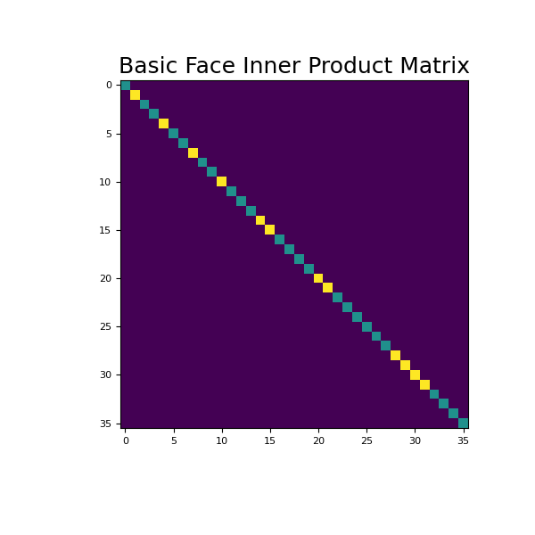
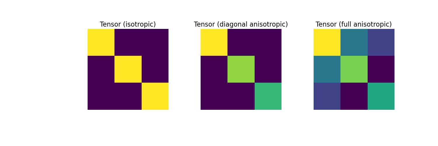
Next, we consider the case where the physical properties of the cells are defined by consistutive relations. For the isotropic, diagonal anisotropic and full tensor cases, we show the physical property tensor for a single cell.
Define 4 constitutive parameters and define the tensor for each cell for isotropic, diagonal and tensor cases.
>>> sig1, sig2, sig3, sig4, sig5, sig6 = 6, 5, 4, 3, 2, 1
>>> sig_iso_tensor = sig1 * np.eye(3)
>>> sig_diag_tensor = np.diag(np.array([sig1, sig2, sig3]))
>>> sig_full_tensor = np.array([
...     [sig1, sig4, sig5],
...     [sig4, sig2, sig6],
...     [sig5, sig6, sig3]
... ])
Then plot matrix entries,
>>> fig = plt.figure(figsize=(15, 5))
>>> ax1 = fig.add_subplot(131)
>>> ax1.imshow(sig_iso_tensor)
>>> ax1.axis('off')
>>> ax1.set_title("Tensor (isotropic)", fontsize=16)
>>> ax2 = fig.add_subplot(132)
>>> ax2.imshow(sig_diag_tensor)
>>> ax2.axis('off')
>>> ax2.set_title("Tensor (diagonal anisotropic)", fontsize=16)
>>> ax3 = fig.add_subplot(133)
>>> ax3.imshow(sig_full_tensor)
>>> ax3.axis('off')
>>> ax3.set_title("Tensor (full anisotropic)", fontsize=16)
>>> plt.show()

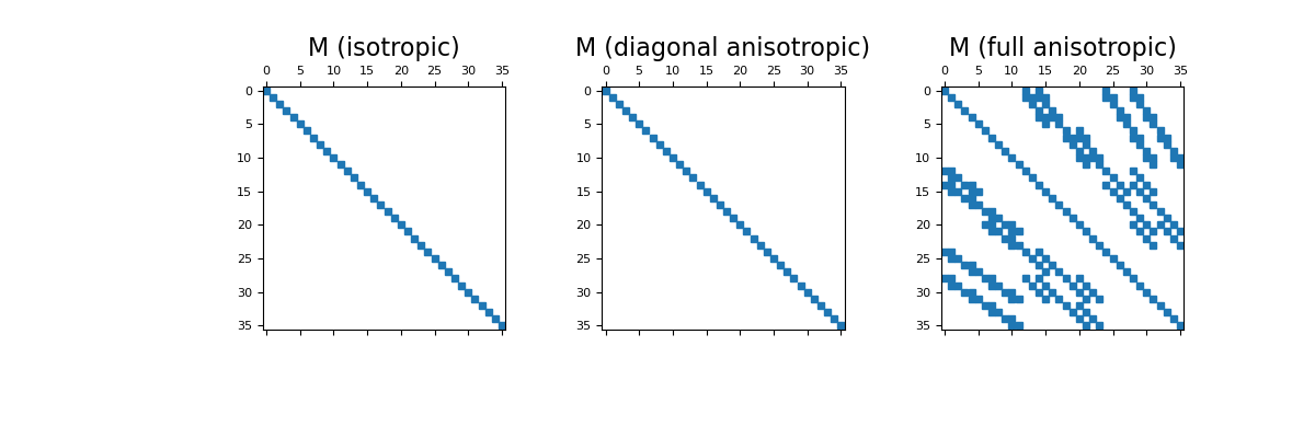
Here, construct and image the face inner product matrices for the isotropic, diagonal anisotropic and full tensor cases. Spy plots are used to demonstrate the sparsity of the inner product matrices.
Isotropic case:
>>> v = np.ones(mesh.nC)
>>> sig = sig1 * v
>>> M1 = mesh.get_face_inner_product(sig)
Diagonal anisotropic case:
>>> sig = np.c_[sig1*v, sig2*v, sig3*v]
>>> M2 = mesh.get_face_inner_product(sig)
Full anisotropic case:
>>> sig = np.tile(np.c_[sig1, sig2, sig3, sig4, sig5, sig6], (mesh.nC, 1))
>>> M3 = mesh.get_face_inner_product(sig)
And then we can plot the sparse representation,
>>> fig = plt.figure(figsize=(12, 4))
>>> ax1 = fig.add_subplot(131)
>>> ax1.spy(M1, ms=5)
>>> ax1.set_title("M (isotropic)", fontsize=16)
>>> ax2 = fig.add_subplot(132)
>>> ax2.spy(M2, ms=5)
>>> ax2.set_title("M (diagonal anisotropic)", fontsize=16)
>>> ax3 = fig.add_subplot(133)
>>> ax3.spy(M3, ms=5)
>>> ax3.set_title("M (full anisotropic)", fontsize=16)
>>> plt.show()
