discretize.utils.inverse_property_tensor#
- discretize.utils.inverse_property_tensor(mesh, tensor, return_matrix=False, **kwargs)[source]#
Construct the inverse of the physical property tensor.
For a given mesh, the input parameter tensor is a
numpy.ndarraydefining the constitutive relationship (e.g. Ohm’s law) between two discrete vector quantities \(\boldsymbol{j}\) and \(\boldsymbol{e}\) living at cell centers. Where \(\boldsymbol{M}\) is the physical property tensor, inverse_property_tensor explicitly constructs the inverse of the physical property tensor \(\boldsymbol{M^{-1}}\) for all cells such that:>>> e = Mi @ j
where the Cartesian components of the discrete vectors are organized according to:
>>> j = np.r_[jx, jy, jz]
>>> e = np.r_[ex, ey, ez]
- Parameters:
- mesh
discretize.base.BaseMesh A mesh
- tensor
numpy.ndarrayorfloat Scalar: A float is entered.
Isotropic: A 1D numpy.ndarray with a property value for every cell.
Anisotropic: A (nCell, dim) numpy.ndarray where each row defines the diagonal-anisotropic property parameters for each cell. nParam = 2 for 2D meshes and nParam = 3 for 3D meshes.
Tensor: A (nCell, nParam) numpy.ndarray where each row defines the full anisotropic property parameters for each cell. nParam = 3 for 2D meshes and nParam = 6 for 3D meshes.
- return_matrixbool,
optional True: the function returns the inverse of the property tensor.
False: the function returns the non-zero elements of the inverse of the property tensor in a numpy.ndarray in the same order as the input argument tensor.
- mesh
- Returns:
numpy.ndarrayorscipy.sparse.coo_matrixIf return_matrix = False, the function outputs the parameters defining the inverse of the property tensor in a numpy.ndarray with the same dimensions as the input argument tensor
If return_natrix = True, the function outputs the inverse of the property tensor as a scipy.sparse.coo_matrix.
Notes
The relationship between a quantity and its response to external stimuli (e.g. Ohm’s law) in each cell can be defined by a scalar function \(\sigma\) in the isotropic case, or by a tensor \(\Sigma\) in the anisotropic case, i.e.:
\[\vec{j} = \sigma \vec{e} \;\;\;\;\;\; \textrm{or} \;\;\;\;\;\; \vec{j} = \Sigma \vec{e}\]where
\[\begin{split}\Sigma = \begin{bmatrix} \sigma_{xx} & \sigma_{xy} & \sigma_{xz} \\ \sigma_{xy} & \sigma_{yy} & \sigma_{yz} \\ \sigma_{xz} & \sigma_{yz} & \sigma_{zz} \end{bmatrix}\end{split}\]Examples
For the 4 classifications allowable (scalar, isotropic, anistropic and tensor), we construct the property tensor on a small 2D mesh. We then construct the inverse of the property tensor and compare.
>>> from discretize.utils import make_property_tensor, inverse_property_tensor
>>> from discretize import TensorMesh
>>> import numpy as np
>>> import matplotlib.pyplot as plt
>>> import matplotlib as mpl
>>> rng = np.random.default_rng(421)
Define a 2D tensor mesh
>>> h = [1., 1., 1.]
>>> mesh = TensorMesh([h, h], origin='00')
Define a physical property for all cases (2D)
>>> sigma_scalar = 4.
>>> sigma_isotropic = rng.integers(1, 10, mesh.nC)
>>> sigma_anisotropic = rng.integers(1, 10, (mesh.nC, 2))
>>> sigma_tensor = rng.integers(1, 10, (mesh.nC, 3))
Construct the property tensor in each case
>>> M_scalar = make_property_tensor(mesh, sigma_scalar)
>>> M_isotropic = make_property_tensor(mesh, sigma_isotropic)
>>> M_anisotropic = make_property_tensor(mesh, sigma_anisotropic)
>>> M_tensor = make_property_tensor(mesh, sigma_tensor)
Construct the inverse property tensor in each case
>>> Minv_scalar = inverse_property_tensor(mesh, sigma_scalar, return_matrix=True)
>>> Minv_isotropic = inverse_property_tensor(mesh, sigma_isotropic, return_matrix=True)
>>> Minv_anisotropic = inverse_property_tensor(mesh, sigma_anisotropic, return_matrix=True)
>>> Minv_tensor = inverse_property_tensor(mesh, sigma_tensor, return_matrix=True)
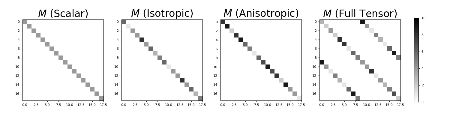
Plot the property tensors.
>>> M_list = [M_scalar, M_isotropic, M_anisotropic, M_tensor]
>>> Minv_list = [Minv_scalar, Minv_isotropic, Minv_anisotropic, Minv_tensor]
>>> case_list = ['Scalar', 'Isotropic', 'Anisotropic', 'Full Tensor']
>>> fig1 = plt.figure(figsize=(15, 4))
>>> ax1 = 4*[None]
>>> for ii in range(0, 4):
...     ax1[ii] = fig1.add_axes([0.05+0.22*ii, 0.05, 0.18, 0.9])
...     ax1[ii].imshow(
...         M_list[ii].todense(), interpolation='none', cmap='binary', vmax=10.
...     )
...     ax1[ii].set_title('$M$ (' + case_list[ii] + ')', fontsize=24)
>>> cax1 = fig1.add_axes([0.92, 0.15, 0.01, 0.7])
>>> norm1 = mpl.colors.Normalize(vmin=0., vmax=10.)
>>> cbar1 = mpl.colorbar.ColorbarBase(
...     cax1, norm=norm1, orientation="vertical", cmap=mpl.cm.binary
... )
>>> plt.show()
(
Source code,png,pdf)
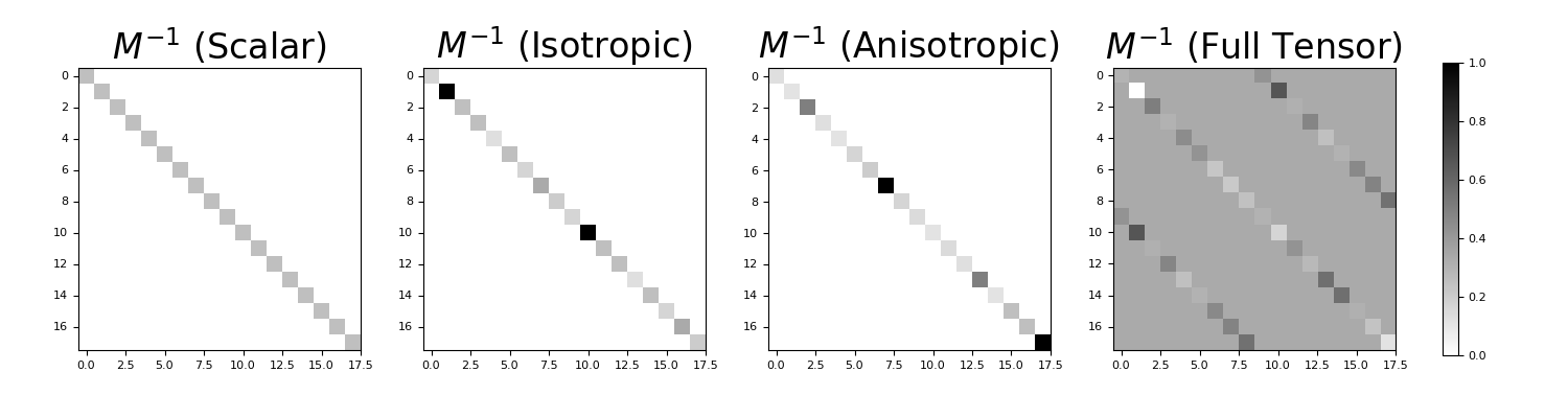
Plot the inverse property tensors.
>>> fig2 = plt.figure(figsize=(15, 4))
>>> ax2 = 4*[None]
>>> for ii in range(0, 4):
...     ax2[ii] = fig2.add_axes([0.05+0.22*ii, 0.05, 0.18, 0.9])
...     ax2[ii].imshow(
...         Minv_list[ii].todense(), interpolation='none', cmap='binary', vmax=1.
...     )
...     ax2[ii].set_title('$M^{-1}$ (' + case_list[ii] + ')', fontsize=24)
>>> cax2 = fig2.add_axes([0.92, 0.15, 0.01, 0.7])
>>> norm2 = mpl.colors.Normalize(vmin=0., vmax=1.)
>>> cbar2 = mpl.colorbar.ColorbarBase(
...     cax2, norm=norm2, orientation="vertical", cmap=mpl.cm.binary
... )
>>> plt.show()
