discretize.utils.interpolation_matrix#
- discretize.utils.interpolation_matrix(locs, x, y=None, z=None)[source]#
Generate interpolation matrix which maps a tensor quantity to a set of locations.
This function generates a sparse matrix for interpolating tensor quantities to a set of specified locations. It uses nD linear interpolation. The user may generate the interpolation matrix for tensor quantities that live on 1D, 2D or 3D tensors. This functionality is frequently used to interpolate quantites from cell centers or nodes to specified locations.
In higher dimensions the ordering of the output has the 1st dimension changing the quickest.
- Parameters:
- locs(
n,dim)numpy.ndarray The locations for the interpolated values. Here n is the number of locations and dim is the dimension (1, 2 or 3)
- x(
nx)numpy.ndarray Vector defining the locations of the tensor along the x-axis
- y(
ny)numpy.ndarray,optional Vector defining the locations of the tensor along the y-axis. Required if
dimis 2.- z(
nz)numpy.ndarray,optional Vector defining the locations of the tensor along the z-axis. Required if
dimis 3.
- locs(
- Returns:
- (
n,nx*ny*nz)scipy.sparse.csr_matrix A sparse matrix which interpolates the tensor quantity on cell centers or nodes to the set of specified locations.
- (
Examples
Here is a 1D example where a function evaluated on a regularly spaced grid is interpolated to a set of random locations. To compare the accuracy, the function is evaluated at the set of random locations.
>>> from discretize.utils import interpolation_matrix
>>> from discretize import TensorMesh
>>> import numpy as np
>>> import matplotlib.pyplot as plt
>>> rng = np.random.default_rng(14)
Create an interpolation matrix
>>> locs = rng.random(50)*0.8+0.1
>>> x = np.linspace(0, 1, 7)
>>> dense = np.linspace(0, 1, 200)
>>> fun = lambda x: np.cos(2*np.pi*x)
>>> Q = interpolation_matrix(locs, x)
Plot original function and interpolation
>>> fig1 = plt.figure(figsize=(5, 3))
>>> ax = fig1.add_axes([0.1, 0.1, 0.8, 0.8])
>>> ax.plot(dense, fun(dense), 'k:', lw=3)
>>> ax.plot(x, fun(x), 'ks', markersize=8)
>>> ax.plot(locs, Q*fun(x), 'go', markersize=4)
>>> ax.plot(locs, fun(locs), 'rs', markersize=4)
>>> ax.legend(
...     [
...         'True Function',
...         'True (discrete loc.)',
...         'Interpolated (computed)',
...         'True (interp. loc.)'
...     ],
...     loc='upper center'
... )
>>> plt.show()
(
Source code,png,pdf)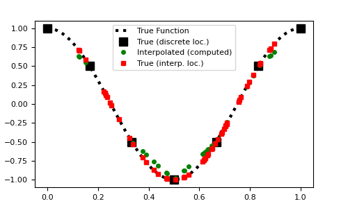
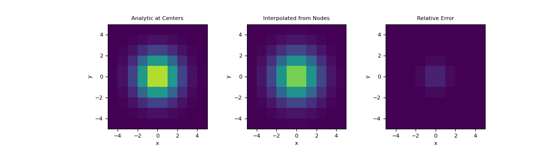
Here, demonstrate a similar example on a 2D mesh using a 2D Gaussian distribution. We interpolate the Gaussian from the nodes to cell centers and examine the relative error.
>>> hx = np.ones(10)
>>> hy = np.ones(10)
>>> mesh = TensorMesh([hx, hy], x0='CC')
>>> def fun(x, y):
...     return np.exp(-(x**2 + y**2)/2**2)
Define the the value at the mesh nodes,
>>> nodes = mesh.nodes
>>> val_nodes = fun(nodes[:, 0], nodes[:, 1])
>>> centers = mesh.cell_centers
>>> A = interpolation_matrix(
...     centers, mesh.nodes_x, mesh.nodes_y
... )
>>> val_interp = A.dot(val_nodes)
Plot the interpolated values, along with the true values at cell centers,
>>> val_centers = fun(centers[:, 0], centers[:, 1])
>>> fig = plt.figure(figsize=(11,3.3))
>>> clim = (0., 1.)
>>> ax1 = fig.add_subplot(131)
>>> ax2 = fig.add_subplot(132)
>>> ax3 = fig.add_subplot(133)
>>> mesh.plot_image(val_centers, ax=ax1, clim=clim)
>>> mesh.plot_image(val_interp, ax=ax2, clim=clim)
>>> mesh.plot_image(val_centers-val_interp, ax=ax3, clim=clim)
>>> ax1.set_title('Analytic at Centers')
>>> ax2.set_title('Interpolated from Nodes')
>>> ax3.set_title('Relative Error')
>>> plt.show()