discretize.TensorMesh.get_interpolation_matrix#
- TensorMesh.get_interpolation_matrix(loc, location_type='cell_centers', zeros_outside=False, **kwargs)[source]#
Construct a linear interpolation matrix from mesh.
This method constructs a linear interpolation matrix from tensor locations (nodes, cell-centers, faces, etc…) on the mesh to a set of arbitrary locations.
- Parameters:
- loc(
n_pts,dim)numpy.ndarray Location of points being to interpolate to. Must have same dimensions as the mesh.
- location_type
str,optional Tensor locations on the mesh being interpolated from. location_type must be one of:
‘Ex’, ‘edges_x’ -> x-component of field defined on x edges
‘Ey’, ‘edges_y’ -> y-component of field defined on y edges
‘Ez’, ‘edges_z’ -> z-component of field defined on z edges
‘Fx’, ‘faces_x’ -> x-component of field defined on x faces
‘Fy’, ‘faces_y’ -> y-component of field defined on y faces
‘Fz’, ‘faces_z’ -> z-component of field defined on z faces
‘N’, ‘nodes’ -> scalar field defined on nodes
‘CC’, ‘cell_centers’ -> scalar field defined on cell centers
‘CCVx’, ‘cell_centers_x’ -> x-component of vector field defined on cell centers
‘CCVy’, ‘cell_centers_y’ -> y-component of vector field defined on cell centers
‘CCVz’, ‘cell_centers_z’ -> z-component of vector field defined on cell centers
- zeros_outsidebool,
optional If False, nearest neighbour is used to compute the interpolate value at locations outside the mesh. If True , values at locations outside the mesh will be zero.
- loc(
- Returns:
- (
n_pts,n_loc_type)scipy.sparse.csr_matrix A sparse matrix which interpolates the specified tensor quantity on mesh to the set of specified locations.
- (
Examples
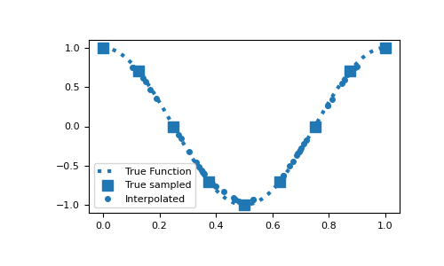
Here is a 1D example where a function evaluated on the nodes is interpolated to a set of random locations. To compare the accuracy, the function is evaluated at the set of random locations.
>>> from discretize import TensorMesh
>>> import numpy as np
>>> import matplotlib.pyplot as plt
>>> rng = np.random.default_rng(14)
>>> locs = rng.random(50)*0.8+0.1
>>> dense = np.linspace(0, 1, 200)
>>> fun = lambda x: np.cos(2*np.pi*x)
>>> hx = 0.125 * np.ones(8)
>>> mesh1D = TensorMesh([hx])
>>> Q = mesh1D.get_interpolation_matrix(locs, 'nodes')
>>> plt.figure(figsize=(5, 3))
>>> plt.plot(dense, fun(dense), ':', c="C0", lw=3, label="True Function")
>>> plt.plot(mesh1D.nodes, fun(mesh1D.nodes), 's', c="C0", ms=8, label="True sampled")
>>> plt.plot(locs, Q*fun(mesh1D.nodes), 'o', ms=4, label="Interpolated")
>>> plt.legend()
>>> plt.show()
(
Source code,png,pdf)
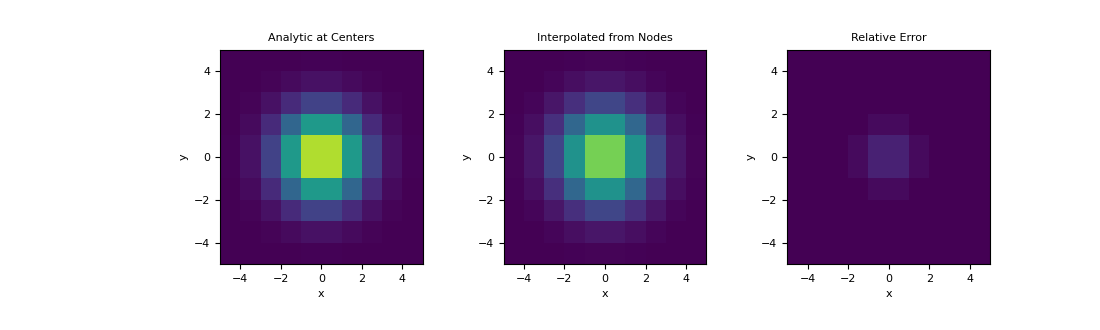
Here, demonstrate a similar example on a 2D mesh using a 2D Gaussian distribution. We interpolate the Gaussian from the nodes to cell centers and examine the relative error.
>>> hx = np.ones(10)
>>> hy = np.ones(10)
>>> mesh2D = TensorMesh([hx, hy], x0='CC')
>>> def fun(x, y):
...     return np.exp(-(x**2 + y**2)/2**2)
>>> nodes = mesh2D.nodes
>>> val_nodes = fun(nodes[:, 0], nodes[:, 1])
>>> centers = mesh2D.cell_centers
>>> val_centers = fun(centers[:, 0], centers[:, 1])
>>> A = mesh2D.get_interpolation_matrix(centers, 'nodes')
>>> val_interp = A.dot(val_nodes)
>>> fig = plt.figure(figsize=(11,3.3))
>>> clim = (0., 1.)
>>> ax1 = fig.add_subplot(131)
>>> ax2 = fig.add_subplot(132)
>>> ax3 = fig.add_subplot(133)
>>> mesh2D.plot_image(val_centers, ax=ax1, clim=clim)
>>> mesh2D.plot_image(val_interp, ax=ax2, clim=clim)
>>> mesh2D.plot_image(val_centers-val_interp, ax=ax3, clim=clim)
>>> ax1.set_title('Analytic at Centers')
>>> ax2.set_title('Interpolated from Nodes')
>>> ax3.set_title('Relative Error')
>>> plt.show()
