discretize.TensorMesh.get_face_inner_product_deriv#
- TensorMesh.get_face_inner_product_deriv(model, do_fast=True, invert_model=False, invert_matrix=False, **kwargs)[source]#
Get a function handle to multiply a vector with derivative of face inner product matrix (or its inverse).
Let \(\mathbf{M}(\mathbf{m})\) be the face inner product matrix constructed with a set of physical property parameters \(\mathbf{m}\) (or its inverse). get_face_inner_product_deriv constructs a function handle
\[\mathbf{F}(\mathbf{u}) = \mathbf{u}^T \, \frac{\partial \mathbf{M}(\mathbf{m})}{\partial \mathbf{m}}\]which accepts any numpy.array \(\mathbf{u}\) of shape (n_faces,). That is, get_face_inner_product_deriv constructs a function handle for computing the dot product between a vector \(\mathbf{u}\) and the derivative of the face inner product matrix (or its inverse) with respect to the property parameters. When computed, \(\mathbf{F}(\mathbf{u})\) returns a
scipy.sparse.csr_matrixof shape (n_faces, n_param).The function handle can be created for isotropic, diagonal isotropic and full tensor physical properties; see notes.
- Parameters:
- model
numpy.ndarray Parameters defining the material properties for every cell in the mesh. Inner product matrices can be constructed for the following cases:
(n_cells)
numpy.ndarray: Isotropic case. model contains a scalar physical property value for each cell.(n_cells, dim)
numpy.ndarray: Diagonal anisotropic case. Columns are orderednp.c_[σ_xx, σ_yy, σ_zz]. This can also a be a 1D array with the same number of total elements in column major order.(n_cells, 3)
numpy.ndarray(dimis 2) or (n_cells, 6)numpy.ndarray(dimis 3) : Full tensor properties case. Columns are orderednp.c_[σ_xx, σ_yy, σ_zz, σ_xy, σ_xz, σ_yz]This can also be a 1D array with the same number of total elements in column major order.
- do_fastbool,
optional Do a faster implementation (if available).
- invert_modelbool,
optional The inverse of model is used as the physical property.
- invert_matrixbool,
optional Returns the inverse of the inner product matrix. The inverse not implemented for full tensor properties.
- model
- Returns:
functionThe function handle \(\mathbf{F}(\mathbf{u})\) which accepts a (
n_faces)numpy.ndarray\(\mathbf{u}\). The function returns a (n_faces,n_params)scipy.sparse.csr_matrix.
Notes
Let \(\mathbf{M}(\mathbf{m})\) be the face inner product matrix (or its inverse) for the set of physical property parameters \(\mathbf{m}\). And let \(\mathbf{u}\) be a discrete quantity that lives on the faces. get_face_inner_product_deriv creates a function handle for computing the following:
\[\mathbf{F}(\mathbf{u}) = \mathbf{u}^T \, \frac{\partial \mathbf{M}(\mathbf{m})}{\partial \mathbf{m}}\]The dimensions of the sparse matrix constructed by computing \(\mathbf{F}(\mathbf{u})\) for some \(\mathbf{u}\) depends on the constitutive relation defined for each cell. These cases are summarized below.
Isotropic Case: The physical property for each cell is defined by a scalar value. Therefore \(\mathbf{m}\) is a (
n_cells)numpy.ndarray. The sparse matrix output by computing \(\mathbf{F}(\mathbf{u})\) has shape (n_faces,n_cells).Diagonal Anisotropic Case: In this case, the physical properties for each cell are defined by a diagonal tensor
\[\begin{split}\Sigma = \begin{bmatrix} \sigma_{xx} & 0 & 0 \\ 0 & \sigma_{yy} & 0 \\ 0 & 0 & \sigma_{zz} \end{bmatrix}\end{split}\]Thus there are
dim * n_cellsphysical property parameters and \(\mathbf{m}\) is a (dim * n_cells)numpy.ndarray. The sparse matrix output by computing \(\mathbf{F}(\mathbf{u})\) has shape (n_faces,dim * n_cells).Full Tensor Case: In this case, the physical properties for each cell are defined by a full tensor
\[\begin{split}\Sigma = \begin{bmatrix} \sigma_{xx} & \sigma_{xy} & \sigma_{xz} \\ \sigma_{xy} & \sigma_{yy} & \sigma_{yz} \\ \sigma_{xz} & \sigma_{yz} & \sigma_{zz} \end{bmatrix}\end{split}\]Thus there are
6 * n_cellsphysical property parameters in 3 dimensions, or3 * n_cellsphysical property parameters in 2 dimensions, and \(\mathbf{m}\) is a (n_params)numpy.ndarray. The sparse matrix output by computing \(\mathbf{F}(\mathbf{u})\) has shape (n_faces,n_params).Examples
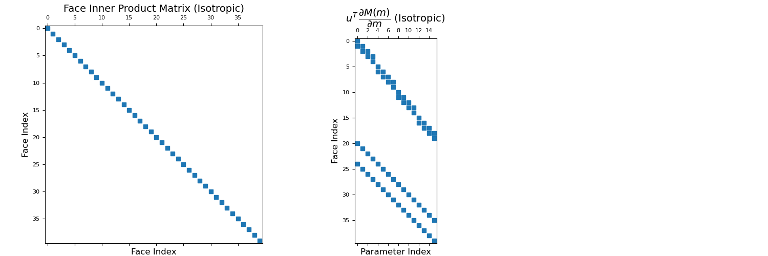
Here, we construct a 4 cell by 4 cell tensor mesh. For our first example we consider isotropic physical properties; that is, the physical properties of each cell are defined a scalar value. We construct the face inner product matrix and visualize it with a spy plot. We then use get_face_inner_product_deriv to construct the function handle \(\mathbf{F}(\mathbf{u})\) and plot the evaluation of this function on a spy plot.
>>> from discretize import TensorMesh
>>> import matplotlib.pyplot as plt
>>> import numpy as np
>>> import matplotlib as mpl
>>> mpl.rcParams.update({'font.size': 14})
>>> rng = np.random.default_rng(45)
>>> mesh = TensorMesh([[(1, 4)], [(1, 4)]])
Define a model, and a random vector to multiply the derivative with, then we grab the respective derivative function and calculate the sparse matrix,
>>> m = rng.random(mesh.nC)  # physical property parameters
>>> u = rng.random(mesh.nF)  # vector of shape (n_faces)
>>> Mf = mesh.get_face_inner_product(m)
>>> F = mesh.get_face_inner_product_deriv(m)  # Function handle
>>> dFdm_u = F(u)
Spy plot for the inner product matrix and its derivative
>>> fig = plt.figure(figsize=(15, 5))
>>> ax1 = fig.add_axes([0.05, 0.05, 0.3, 0.85])
>>> ax1.spy(Mf, ms=6)
>>> ax1.set_title("Face Inner Product Matrix (Isotropic)", fontsize=14, pad=5)
>>> ax1.set_xlabel("Face Index", fontsize=12)
>>> ax1.set_ylabel("Face Index", fontsize=12)
>>> ax2 = fig.add_axes([0.43, 0.05, 0.17, 0.8])
>>> ax2.spy(dFdm_u, ms=6)
>>> ax2.set_title(
...     r"$u^T \, \dfrac{\partial M(m)}{\partial m}$ (Isotropic)",
...     fontsize=14, pad=5
... )
>>> ax2.set_xlabel("Parameter Index", fontsize=12)
>>> ax2.set_ylabel("Face Index", fontsize=12)
>>> plt.show()
(
Source code,png,pdf)
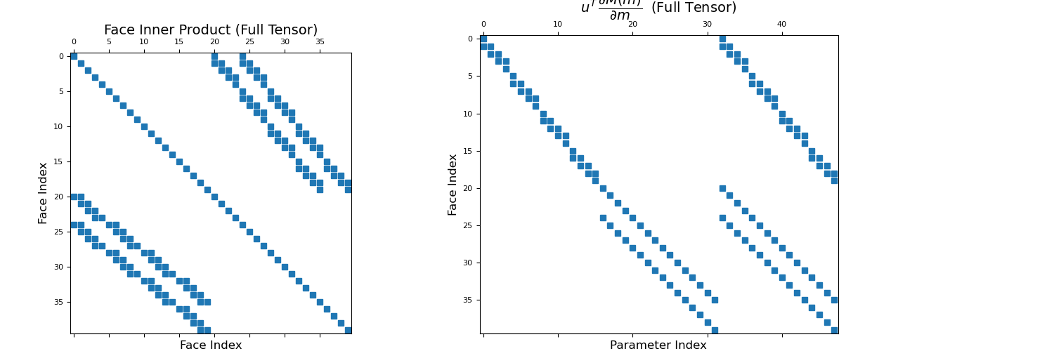
For our second example, the physical properties on the mesh are fully anisotropic; that is, the physical properties of each cell are defined by a tensor with parameters \(\sigma_1\), \(\sigma_2\) and \(\sigma_3\). Once again we construct the face inner product matrix and visualize it with a spy plot. We then use get_face_inner_product_deriv to construct the function handle \(\mathbf{F}(\mathbf{u})\) and plot the evaluation of this function on a spy plot.
>>> m = rng.random((mesh.nC, 3))  # anisotropic physical property parameters
>>> u = rng.random(mesh.nF)     # vector of shape (n_faces)
>>> Mf = mesh.get_face_inner_product(m)
>>> F = mesh.get_face_inner_product_deriv(m)  # Function handle
>>> dFdm_u = F(u)
Plot the anisotropic inner product matrix and its derivative matrix,
>>> fig = plt.figure(figsize=(15, 5))
>>> ax1 = fig.add_axes([0.05, 0.05, 0.3, 0.8])
>>> ax1.spy(Mf, ms=6)
>>> ax1.set_title("Face Inner Product (Full Tensor)", fontsize=14, pad=5)
>>> ax1.set_xlabel("Face Index", fontsize=12)
>>> ax1.set_ylabel("Face Index", fontsize=12)
>>> ax2 = fig.add_axes([0.4, 0.05, 0.45, 0.85])
>>> ax2.spy(dFdm_u, ms=6)
>>> ax2.set_title(
...     r"$u^T \, \dfrac{\partial M(m)}{\partial m} \;$ (Full Tensor)",
...     fontsize=14, pad=5
... )
>>> ax2.set_xlabel("Parameter Index", fontsize=12)
>>> ax2.set_ylabel("Face Index", fontsize=12)
>>> plt.show()
