discretize.TensorMesh.get_edge_inner_product_line

TensorMesh.get_edge_inner_product_line(model=None, invert_model=False, invert_matrix=False, **kwargs)

Generate the edge inner product line matrix or its inverse.

This method generates the inner product line matrix (or its inverse) when discrete variables are defined on mesh edges. It is also capable of constructing the inner product line matrix when diagnostic properties (e.g. integrated conductance) are defined on mesh edges. For a comprehensive description of the inner product line matrices that can be constructed with get_edge_inner_product_line, see Notes.

Parameters:

modelNone or numpy.ndarray

Parameters defining the diagnostic property for every edge in the mesh. Inner product line matrices can be constructed for the following cases:

• None : returns the basic inner product line matrix

• (n_edges) numpy.ndarray : returns inner product line matrix for an isotropic model. The array contains a scalar diagnostic property value for each edge.

invert_modelbool, optional

The inverse of model is used as the diagnostic property.

invert_matrixbool, optional

Returns the inverse of the inner product line matrix. The inverse not implemented for full tensor properties.

Returns:

(n_edges, n_edges) scipy.sparse.csr_matrix

inner product line matriz

Notes

For continuous vector quantities \(\vec{u}\) and \(\vec{w}\), and scalar physical property distribution \(\sigma\), we define the following inner product:

\[\langle \vec{u}, \sigma \vec{w} \rangle = \int_\Omega \, \vec{u} \cdot \sigma \vec{v} \, dv\]

If the material property is distributed over a set of lines \(\ell_i\) with cross-sectional area \(a\), we can define a diagnostic property value \(\lambda = \sigma a\). And the inner-product can be approximated by a set of line integrals as follows:

\[\langle \vec{u}, \sigma \vec{w} \rangle = \sum_i \int_{\ell_i} \, \vec{u} \cdot \lambda \vec{v} \, ds\]

Let \(\vec{u}\) and \(\vec{w}\) have discrete representations \(\mathbf{u}\) and \(\mathbf{w}\) that live on the edges. Assuming the contribution of vector components perpendicular to the lines are negligible compared to parallel components, get_edge_inner_product_line constructs the inner product matrix \(\mathbf{M_\lambda}\) (or its inverse \(\mathbf{M_\lambda^{-1}}\)) such that:

\[\sum_i \int_{\ell_i} \, \vec{u} \cdot \lambda \vec{v} \, ds \approx \sum_i \int_{\ell_i} \, \vec{u}_\parallel \cdot \lambda \vec{v}_\parallel \, ds = \mathbf{u^T \, M_\lambda \, w}\]

where the diagnostic properties on mesh edges (i.e. the model) are stored within an array of the form:

\[\begin{split}\boldsymbol{\lambda} = \begin{bmatrix} \boldsymbol{\lambda_x} \\ \boldsymbol{\lambda_y} \\ \boldsymbol{\lambda_z} \end{bmatrix}\end{split}\]

Examples

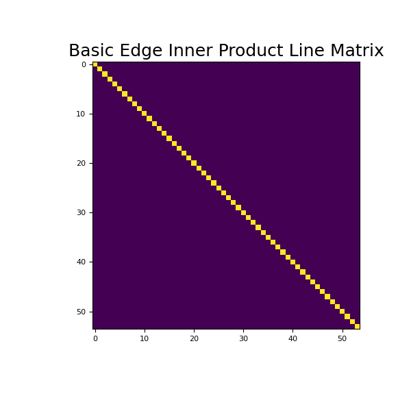
Here we provide an example of edge inner product line matrix. For simplicity, we will work on a 2 x 2 x 2 tensor mesh. As seen below, we begin by constructing and imaging the basic edge inner product line matrix.

>>> from discretize import TensorMesh
>>> import matplotlib.pyplot as plt
>>> import numpy as np

>>> h = np.ones(2)
>>> mesh = TensorMesh([h, h, h])
>>> Me = mesh.get_edge_inner_product_line()

>>> fig = plt.figure(figsize=(6, 6))
>>> ax = fig.add_subplot(111)
>>> ax.imshow(Me.todense())
>>> ax.set_title('Basic Edge Inner Product Line Matrix', fontsize=18)
>>> plt.show()

(Source code, png, pdf)

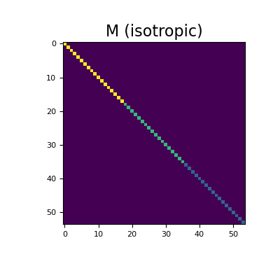
Next, we consider the case where the physical properties are defined by diagnostic properties on mesh edges. For the isotropic case, we show the physical property tensor for a single cell.

Define the diagnostic property values for x, y and z faces.

>>> tau_x, tau_y, tau_z = 3, 2, 1

Here construct and image the edge inner product line matrix for the isotropic case. Spy plots are used to demonstrate the sparsity of the matrix.

>>> tau = np.r_[
>>>     tau_x * np.ones(mesh.n_edges_x),
>>>     tau_y * np.ones(mesh.n_edges_y),
>>>     tau_z * np.ones(mesh.n_edges_z)
>>> ]
>>> M = mesh.get_edge_inner_product_line(tau)

Then plot the sparse representation,

>>> fig = plt.figure(figsize=(4, 4))
>>> ax1 = fig.add_subplot(111)
>>> ax1.imshow(M.todense())
>>> ax1.set_title("M (isotropic)", fontsize=16)
>>> plt.show()

(png, pdf)