discretize.CurvilinearMesh.plot_slice#
- CurvilinearMesh.plot_slice(v, v_type='CC', normal='Z', ind=None, slice_loc=None, grid=False, view='real', ax=None, clim=None, show_it=False, pcolor_opts=None, stream_opts=None, grid_opts=None, range_x=None, range_y=None, sample_grid=None, stream_threshold=None, stream_thickness=None, **kwargs)[source]#
Plot a slice of fields on the given 3D mesh.
- Parameters:
- v
numpy.ndarray values to plot
- v_type{‘CC’,’CCV’, ‘N’, ‘F’, ‘Fx’, ‘Fy’, ‘Fz’, ‘E’, ‘Ex’, ‘Ey’, ‘Ez’},
ortupleoftheseoptions Where the values of v are defined.
- normal{‘Z’, ‘X’, ‘Y’}
Normal direction of slicing plane.
- ind
None,optional index along dimension of slice. Defaults to the center index.
- slice_loc
None,optional Value along dimension of slice. Defaults to the center of the mesh.
- view{‘real’, ‘imag’, ‘abs’, ‘vec’}
How to view the array.
- ax
matplotlib.axes.Axes,optional The axes to draw on. None produces a new Axes. Must be None if
v_typeis a tuple.- clim
tupleoffloat,optional length 2 tuple of (vmin, vmax) for the color limits
- range_x, range_y
tupleoffloat,optional length 2 tuple of (min, max) for the bounds of the plot axes.
- pcolor_opts
dict,optional Arguments passed on to
pcolormesh- gridbool,
optional Whether to plot the edges of the mesh cells.
- grid_opts
dict,optional If
gridis true, arguments passed on toplotfor the edges- sample_grid
tupleofnumpy.ndarray,optional If
view== ‘vec’, mesh cell widths (hx, hy) to interpolate onto for vector plotting- stream_opts
dict,optional If
view== ‘vec’, arguments passed on tostreamplot- stream_thickness
float,optional If
view== ‘vec’, linewidth forstreamplot- stream_threshold
float,optional If
view== ‘vec’, only plots vectors with magnitude above this threshold- show_itbool,
optional Whether to call plt.show()
- v
Examples
Plot a slice of a 3D TensorMesh solution to a Laplace’s equaiton.
First build the mesh:
>>> from matplotlib import pyplot as plt
>>> import discretize
>>> from scipy.sparse.linalg import spsolve
>>> hx = [(5, 2, -1.3), (2, 4), (5, 2, 1.3)]
>>> hy = [(2, 2, -1.3), (2, 6), (2, 2, 1.3)]
>>> hz = [(2, 2, -1.3), (2, 6), (2, 2, 1.3)]
>>> M = discretize.TensorMesh([hx, hy, hz])
then build the necessary parts of the PDE:
>>> q = np.zeros(M.vnC)
>>> q[[4, 4], [4, 4], [2, 6]]=[-1, 1]
>>> q = discretize.utils.mkvc(q)
>>> A = M.face_divergence * M.cell_gradient
>>> b = spsolve(A, q)
and finaly, plot the vector values of the result, which are defined on faces
>>> M.plot_slice(M.cell_gradient*b, 'F', view='vec', grid=True, pcolor_opts={'alpha':0.8})
>>> plt.show()
(
Source code,png,pdf)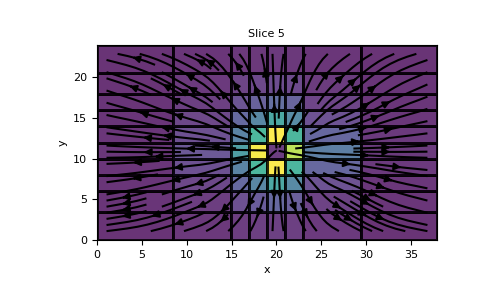
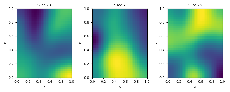
We can use the slice_loc kwarg to tell `plot_slice where to slice the mesh. Let’s create a mesh with a random model and plot slice of it. The slice_loc kwarg automatically determines the indices for slicing the mesh along a plane with the given normal.
>>> M = discretize.TensorMesh([32, 32, 32])
>>> v = discretize.utils.random_model(M.vnC, random_seed=789).reshape(-1, order='F')
>>> x_slice, y_slice, z_slice = 0.75, 0.25, 0.9
>>> plt.figure(figsize=(7.5, 3))
>>> ax = plt.subplot(131)
>>> M.plot_slice(v, normal='X', slice_loc=x_slice, ax=ax)
>>> ax = plt.subplot(132)
>>> M.plot_slice(v, normal='Y', slice_loc=y_slice, ax=ax)
>>> ax = plt.subplot(133)
>>> M.plot_slice(v, normal='Z', slice_loc=z_slice, ax=ax)
>>> plt.tight_layout()
>>> plt.show()
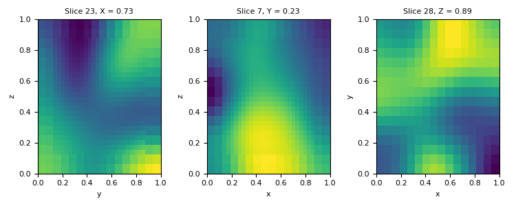
This also works for TreeMesh. We create a mesh here that is refined within three boxes, along with a base level of refinement.
>>> TM = discretize.TreeMesh([32, 32, 32])
>>> TM.refine(3, finalize=False)
>>> BSW = [[0.25, 0.25, 0.25], [0.15, 0.15, 0.15], [0.1, 0.1, 0.1]]
>>> TNE = [[0.75, 0.75, 0.75], [0.85, 0.85, 0.85], [0.9, 0.9, 0.9]]
>>> levels = [6, 5, 4]
>>> TM.refine_box(BSW, TNE, levels)
>>> v_TM = discretize.utils.volume_average(M, TM, v)
>>> plt.figure(figsize=(7.5, 3))
>>> ax = plt.subplot(131)
>>> TM.plot_slice(v_TM, normal='X', slice_loc=x_slice, ax=ax)
>>> ax = plt.subplot(132)
>>> TM.plot_slice(v_TM, normal='Y', slice_loc=y_slice, ax=ax)
>>> ax = plt.subplot(133)
>>> TM.plot_slice(v_TM, normal='Z', slice_loc=z_slice, ax=ax)
>>> plt.tight_layout()
>>> plt.show()
