discretize.CurvilinearMesh.cell_gradient#
- property CurvilinearMesh.cell_gradient#
Cell gradient operator (cell centers to faces).
This property constructs the 2nd order numerical gradient operator that maps from cell centers to faces. The operator is a sparse matrix \(\mathbf{G_c}\) that can be applied as a matrix-vector product to a discrete scalar quantity \(\boldsymbol{\phi}\) that lives at the cell centers; i.e.:
grad_phi = Gc @ phi
By default, the operator assumes zero-Neumann boundary conditions on the scalar quantity. Before calling cell_gradient however, the user can set a mix of zero Dirichlet and zero Neumann boundary conditions using
set_cell_gradient_BC. When cell_gradient is called, the boundary conditions are enforced for the gradient operator. Once constructed, the operator is stored as a property of the mesh. See notes.This operator is defined mostly as a helper property, and is not necessarily recommended to use when solving PDE’s.
- Returns:
- (
n_faces,n_cells)scipy.sparse.csr_matrix The numerical gradient operator from cell centers to faces
- (
Notes
In continuous space, the gradient operator is defined as:
\[\vec{u} = \nabla \phi = \frac{\partial \phi}{\partial x}\hat{x} + \frac{\partial \phi}{\partial y}\hat{y} + \frac{\partial \phi}{\partial z}\hat{z}\]Where \(\boldsymbol{\phi}\) is the discrete representation of the continuous variable \(\phi\) at cell centers and \(\mathbf{u}\) is the discrete representation of \(\vec{u}\) on the faces, cell_gradient constructs a discrete linear operator \(\mathbf{G_c}\) such that:
\[\mathbf{u} = \mathbf{G_c} \, \boldsymbol{\phi}\]Second order ghost points are used to enforce boundary conditions and map appropriately to boundary faces. Along each axes direction, we are effectively computing the derivative by taking the difference between the values at adjacent cell centers and dividing by their distance.
Examples
Below, we demonstrate how to set boundary conditions for the cell gradient operator, construct the cell gradient operator and apply it to a discrete scalar quantity. The mapping of the operator and its sparsity is also illustrated. Our example is carried out on a 2D mesh but it can be done equivalently for a 3D mesh.
We start by importing the necessary packages and modules.
>>> from discretize import TensorMesh
>>> import numpy as np
>>> import matplotlib.pyplot as plt
>>> import matplotlib as mpl
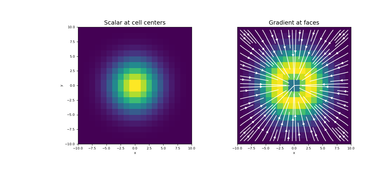
We then construct a mesh and define a scalar function at cell centers which is zero on the boundaries (zero Dirichlet).
Create a uniform grid
>>> h = np.ones(20)
>>> mesh = TensorMesh([h, h], "CC")
Create a discrete scalar on nodes
>>> centers = mesh.cell_centers
>>> phi = np.exp(-(centers[:, 0] ** 2 + centers[:, 1] ** 2) / 4 ** 2)
Once the operator is created, the gradient is performed as a matrix-vector product.
Construct the gradient operator and apply to vector
>>> Gc = mesh.cell_gradient
>>> grad_phi = Gc @ phi
Plot the results
>>> fig = plt.figure(figsize=(13, 6))
>>> ax1 = fig.add_subplot(121)
>>> mesh.plot_image(phi, ax=ax1)
>>> ax1.set_title("Scalar at cell centers", fontsize=14)
>>> ax2 = fig.add_subplot(122)
>>> mesh.plot_image(
...     grad_phi, ax=ax2, v_type="F", view="vec",
...     stream_opts={"color": "w", "density": 1.0}
... )
>>> ax2.set_yticks([])
>>> ax2.set_ylabel("")
>>> ax2.set_title("Gradient at faces", fontsize=14)
>>> plt.show()
(
Source code,png,pdf)
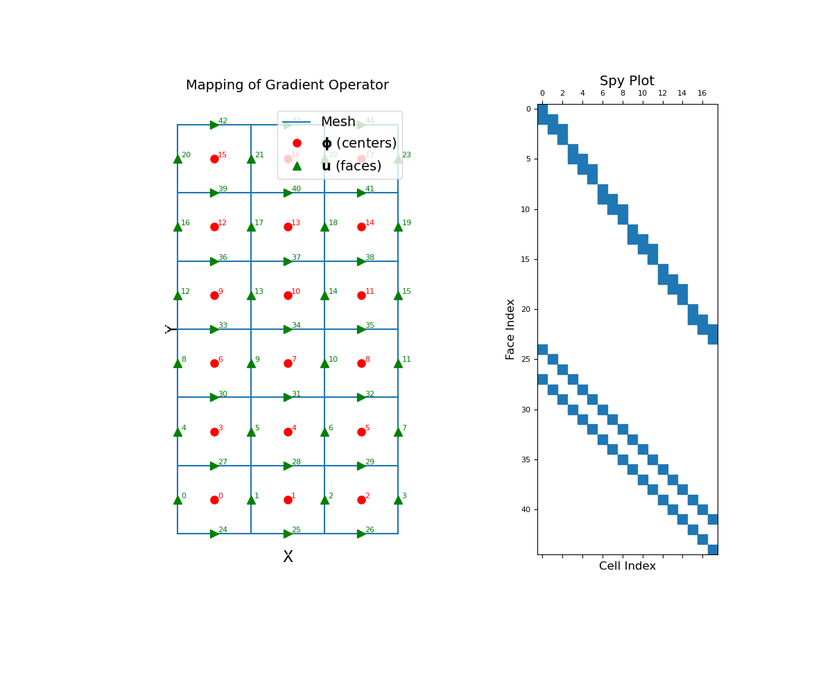
The cell gradient operator is a sparse matrix that maps from cell centers to faces. To demonstrate this, we construct a small 2D mesh. We then show the ordering of the elements in the original discrete quantity \(\boldsymbol{\phi}\) and its discrete gradient as well as a spy plot.
>>> mesh = TensorMesh([[(1, 3)], [(1, 6)]])
>>> mesh.set_cell_gradient_BC('dirichlet')
>>> fig = plt.figure(figsize=(12, 10))
>>> ax1 = fig.add_subplot(121)
>>> mesh.plot_grid(ax=ax1)
>>> ax1.set_title("Mapping of Gradient Operator", fontsize=14, pad=15)
>>> ax1.plot(mesh.cell_centers[:, 0], mesh.cell_centers[:, 1], "ro", markersize=8)
>>> for ii, loc in zip(range(mesh.nC), mesh.cell_centers):
...     ax1.text(loc[0] + 0.05, loc[1] + 0.02, "{0:d}".format(ii), color="r")
>>> ax1.plot(mesh.faces_x[:, 0], mesh.faces_x[:, 1], "g^", markersize=8)
>>> for ii, loc in zip(range(mesh.nFx), mesh.faces_x):
...     ax1.text(loc[0] + 0.05, loc[1] + 0.02, "{0:d}".format(ii), color="g")
>>> ax1.plot(mesh.faces_y[:, 0], mesh.faces_y[:, 1], "g>", markersize=8)
>>> for ii, loc in zip(range(mesh.nFy), mesh.faces_y):
...     ax1.text(loc[0] + 0.05, loc[1] + 0.02, "{0:d}".format((ii + mesh.nFx)), color="g")
>>> ax1.set_xticks([])
>>> ax1.set_yticks([])
>>> ax1.spines['bottom'].set_color('white')
>>> ax1.spines['top'].set_color('white')
>>> ax1.spines['left'].set_color('white')
>>> ax1.spines['right'].set_color('white')
>>> ax1.set_xlabel('X', fontsize=16, labelpad=-5)
>>> ax1.set_ylabel('Y', fontsize=16, labelpad=-15)
>>> ax1.legend(
...     ['Mesh', r'$\mathbf{\phi}$ (centers)', r'$\mathbf{u}$ (faces)'],
...     loc='upper right', fontsize=14
... )
>>> ax2 = fig.add_subplot(122)
>>> ax2.spy(mesh.cell_gradient)
>>> ax2.set_title("Spy Plot", fontsize=14, pad=5)
>>> ax2.set_ylabel("Face Index", fontsize=12)
>>> ax2.set_xlabel("Cell Index", fontsize=12)
>>> plt.show()
