discretize.operators.DiffOperators.average_edge_z_to_cell#
- property DiffOperators.average_edge_z_to_cell#
Averaging operator from z-edges to cell centers (scalar quantities).
This property constructs a 2nd order averaging operator that maps scalar quantities from z-edges to cell centers. This averaging operator is used when a discrete scalar quantity defined on z-edges must be projected to cell centers. Once constructed, the operator is stored permanently as a property of the mesh. See notes.
- Returns:
- (
n_cells,n_edges_z)scipy.sparse.csr_matrix The scalar averaging operator from z-edges to cell centers
- (
Notes
Let \(\boldsymbol{\phi_z}\) be a discrete scalar quantity that lives on z-edges. average_edge_z_to_cell constructs a discrete linear operator \(\mathbf{A_{zc}}\) that projects \(\boldsymbol{\phi_z}\) to cell centers, i.e.:
\[\boldsymbol{\phi_c} = \mathbf{A_{zc}} \, \boldsymbol{\phi_z}\]where \(\boldsymbol{\phi_c}\) approximates the value of the scalar quantity at cell centers. For each cell, we are simply averaging the values defined on its z-edges. The operation is implemented as a matrix vector product, i.e.:
phi_c = Azc @ phi_z
Examples
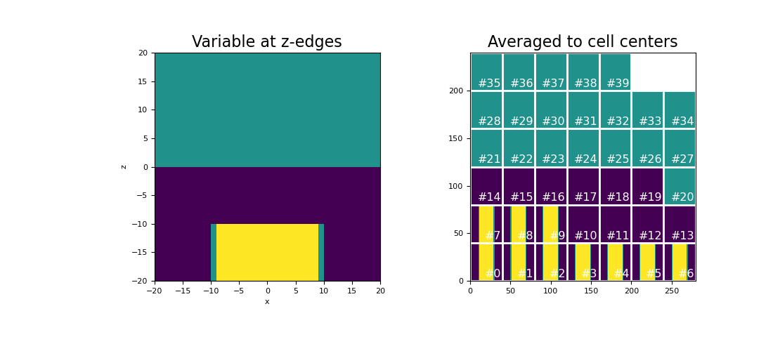
Here we compute the values of a scalar function on the z-edges. We then create an averaging operator to approximate the function at cell centers. We choose to define a scalar function that is strongly discontinuous in some places to demonstrate how the averaging operator will smooth out discontinuities.
We start by importing the necessary packages and defining a mesh.
>>> from discretize import TensorMesh
>>> import numpy as np
>>> import matplotlib.pyplot as plt
>>> h = np.ones(40)
>>> mesh = TensorMesh([h, h, h], x0="CCC")
The we create a scalar variable on z-edges,
>>> phi_z = np.zeros(mesh.nEz)
>>> xyz = mesh.edges_z
>>> phi_z[(xyz[:, 2] > 0)] = 25.0
>>> phi_z[(xyz[:, 2] < -10.0) & (xyz[:, 0] > -10.0) & (xyz[:, 0] < 10.0)] = 50.0
Next, we construct the averaging operator and apply it to the discrete scalar quantity to approximate the value at cell centers. We plot the original scalar and its average at cell centers for a slice at y=0.
>>> Azc = mesh.average_edge_z_to_cell
>>> phi_c = Azc @ phi_z
Plot the results,
>>> fig = plt.figure(figsize=(11, 5))
>>> ax1 = fig.add_subplot(121)
>>> v = np.r_[np.zeros(mesh.nEx+mesh.nEy), phi_z]  # create vector for plotting
>>> mesh.plot_slice(v, ax=ax1, normal='Y', slice_loc=0, v_type="Ez")
>>> ax1.set_title("Variable at z-edges", fontsize=16)
>>> ax2 = fig.add_subplot(122)
>>> mesh.plot_image(phi_c, ax=ax2, normal='Y', slice_loc=0, v_type="CC")
>>> ax2.set_title("Averaged to cell centers", fontsize=16)
>>> plt.show()
(
Source code,png,pdf)
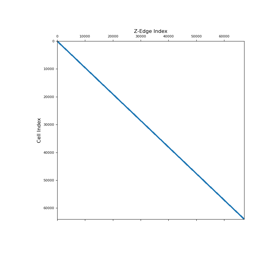
Below, we show a spy plot illustrating the sparsity and mapping of the operator
>>> fig = plt.figure(figsize=(9, 9))
>>> ax1 = fig.add_subplot(111)
>>> ax1.spy(Azc, ms=1)
>>> ax1.set_title("Z-Edge Index", fontsize=12, pad=5)
>>> ax1.set_ylabel("Cell Index", fontsize=12)
>>> plt.show()
