discretize.CylindricalMesh.cell_gradient_x#
- property CylindricalMesh.cell_gradient_x#
X-derivative operator (cell centers to x-faces).
This property constructs an x-derivative operator that acts on cell centered quantities; i.e. the x-component of the cell gradient operator. When applied, the x-derivative is mapped to x-faces. The operator is a sparse matrix \(\mathbf{G_x}\) that can be applied as a matrix-vector product to a cell centered quantity \(\boldsymbol{\phi}\), i.e.:
grad_phi_x = Gx @ phi
By default, the operator assumes zero-Neumann boundary conditions on the scalar quantity. Before calling cell_gradient_x however, the user can set a mix of zero Dirichlet and zero Neumann boundary conditions using
set_cell_gradient_BC. When cell_gradient_x is called, the boundary conditions are enforced for the differencing operator.- Returns:
- (
n_faces_x,n_cells)scipy.sparse.csr_matrix X-derivative operator (x-component of the cell gradient)
- (
Examples
Below, we demonstrate how to set boundary conditions for the x-component cell gradient, construct the operator and apply it to a discrete scalar quantity. The mapping of the operator and its sparsity is also illustrated. Our example is carried out on a 2D mesh but it can be done equivalently for a 3D mesh.
We start by importing the necessary packages and modules.
>>> from discretize import TensorMesh
>>> import numpy as np
>>> import matplotlib.pyplot as plt
>>> import matplotlib as mpl
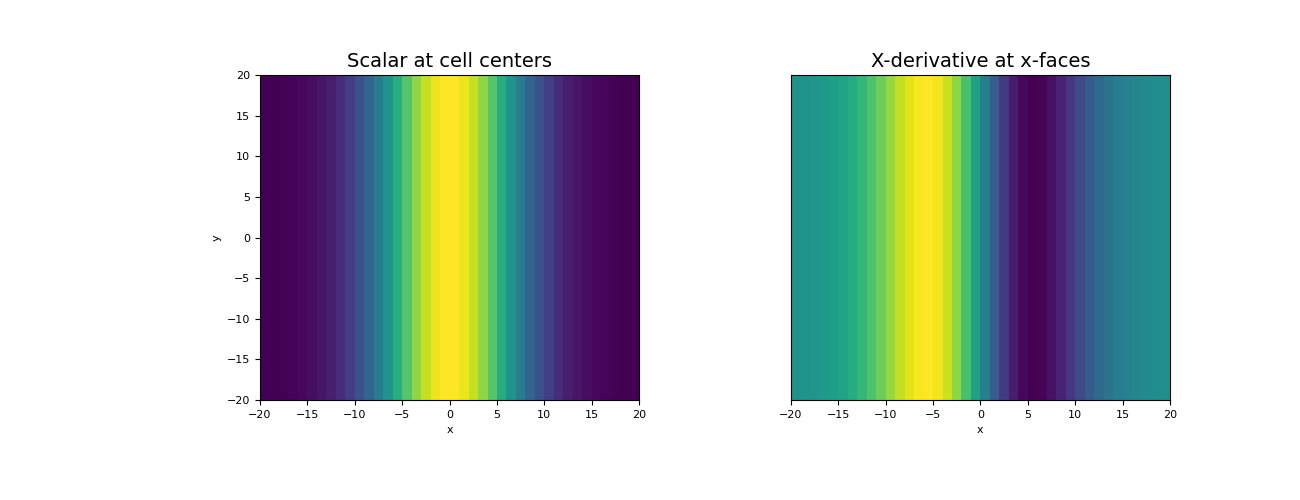
We then construct a mesh and define a scalar function at cell centers.
>>> h = np.ones(40)
>>> mesh = TensorMesh([h, h], "CC")
>>> centers = mesh.cell_centers
>>> phi = np.exp(-(centers[:, 0] ** 2) / 8** 2)
Before constructing the operator, we must define the boundary conditions; zero Neumann for our example. Even though we are only computing the derivative along x, we define boundary conditions for all boundary faces. Once the operator is created, it is applied as a matrix-vector product.
>>> mesh.set_cell_gradient_BC(['neumann', 'neumann'])
>>> Gx = mesh.stencil_cell_gradient_x
>>> grad_phi_x = Gx @ phi
Now we plot the original scalar, and the x-derivative.
>>> fig = plt.figure(figsize=(13, 5))
>>> ax1 = fig.add_subplot(121)
>>> mesh.plot_image(phi, ax=ax1)
>>> ax1.set_title("Scalar at cell centers", fontsize=14)
>>> ax2 = fig.add_subplot(122)
>>> v = np.r_[grad_phi_x, np.zeros(mesh.nFy)]  # Define vector for plotting fun
>>> mesh.plot_image(v, ax=ax2, v_type="Fx")
>>> ax2.set_yticks([])
>>> ax2.set_ylabel("")
>>> ax2.set_title("X-derivative at x-faces", fontsize=14)
>>> plt.show()
(
Source code,png,pdf)
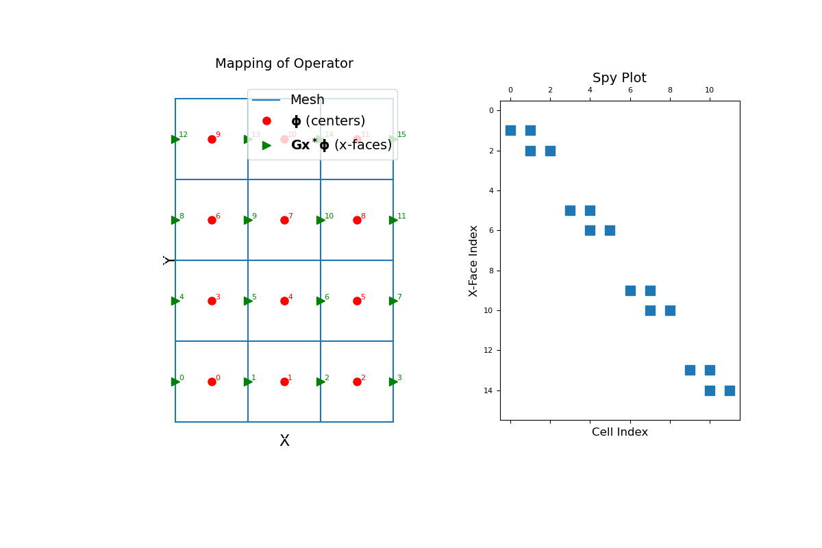
The operator is a sparse x-derivative matrix that maps from cell centers to x-faces. To demonstrate this, we construct a small 2D mesh. We then show the ordering of the elements and a spy plot.
>>> mesh = TensorMesh([[(1, 3)], [(1, 4)]])
>>> mesh.set_cell_gradient_BC('neumann')
>>> fig = plt.figure(figsize=(12, 8))
>>> ax1 = fig.add_subplot(121)
>>> mesh.plot_grid(ax=ax1)
>>> ax1.set_title("Mapping of Operator", fontsize=14, pad=15)
>>> ax1.plot(mesh.cell_centers[:, 0], mesh.cell_centers[:, 1], "ro", markersize=8)
>>> for ii, loc in zip(range(mesh.nC), mesh.cell_centers):
...     ax1.text(loc[0] + 0.05, loc[1] + 0.02, "{0:d}".format(ii), color="r")
>>> ax1.plot(mesh.faces_x[:, 0], mesh.faces_x[:, 1], "g>", markersize=8)
>>> for ii, loc in zip(range(mesh.nFx), mesh.faces_x):
...     ax1.text(loc[0] + 0.05, loc[1] + 0.02, "{0:d}".format(ii), color="g")
>>> ax1.set_xticks([])
>>> ax1.set_yticks([])
>>> ax1.spines['bottom'].set_color('white')
>>> ax1.spines['top'].set_color('white')
>>> ax1.spines['left'].set_color('white')
>>> ax1.spines['right'].set_color('white')
>>> ax1.set_xlabel('X', fontsize=16, labelpad=-5)
>>> ax1.set_ylabel('Y', fontsize=16, labelpad=-15)
>>> ax1.legend(
...     ['Mesh', r'$\mathbf{\phi}$ (centers)', r'$\mathbf{Gx^* \phi}$ (x-faces)'],
...     loc='upper right', fontsize=14
... )
>>> ax2 = fig.add_subplot(122)
>>> ax2.spy(mesh.cell_gradient_x)
>>> ax2.set_title("Spy Plot", fontsize=14, pad=5)
>>> ax2.set_ylabel("X-Face Index", fontsize=12)
>>> ax2.set_xlabel("Cell Index", fontsize=12)
>>> plt.show()