Overview of Mesh Types

Here we provide an overview of mesh types and define some terminology. Separate tutorials have been provided for each mesh type.

import numpy as np
import discretize
import matplotlib.pyplot as plt

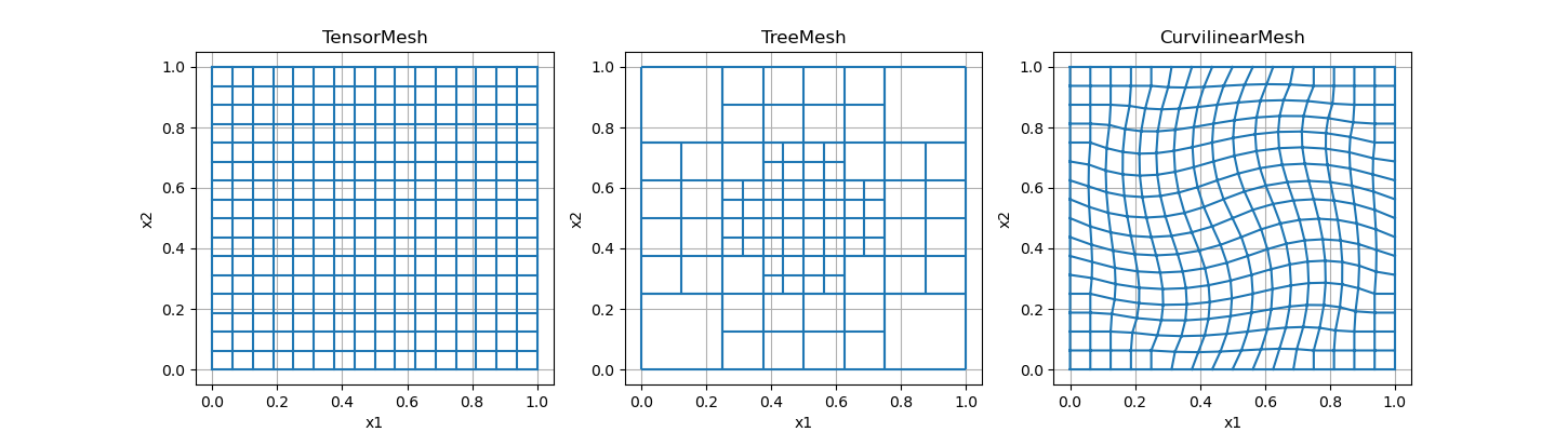
General Categories of Meshes

The three main types of meshes in discretize are

• Tensor meshes (discretize.TensorMesh); which includes cylindrical meshes (discretize.CylindricalMesh)

• Tree meshes (discretize.TreeMesh): also referred to as QuadTree or OcTree meshes

• Curvilinear meshes (discretize.CurviMesh): also referred to as logically rectangular non-orthogonal

Examples for each mesh type are shown below.

ncx = 16  # number of cells in the x-direction
ncy = 16  # number of cells in the y-direction

# create a tensor mesh
tensor_mesh = discretize.TensorMesh([ncx, ncy])

# create a tree mesh and refine some of the cells
tree_mesh = discretize.TreeMesh([ncx, ncy])


def refine(cell):
    if np.sqrt(((np.r_[cell.center] - 0.5) ** 2).sum()) < 0.2:
        return 4
    return 2


tree_mesh.refine(refine)

# create a curvilinear mesh
curvi_mesh = discretize.CurvilinearMesh(
    discretize.utils.example_curvilinear_grid([ncx, ncy], "rotate")
)

# Plot
fig, axes = plt.subplots(1, 3, figsize=(14.5, 4))
tensor_mesh.plot_grid(ax=axes[0])
axes[0].set_title("TensorMesh")

tree_mesh.plot_grid(ax=axes[1])
axes[1].set_title("TreeMesh")

curvi_mesh.plot_grid(ax=axes[2])
axes[2].set_title("CurvilinearMesh")

Text(0.5, 1.0, 'CurvilinearMesh')

Variable Locations and Terminology

When solving differential equations on a numerical grid, variables can be defined on:

• nodes

• cell centers

• cell faces

• cell edges

Below we show an example for a 2D tensor mesh.

hx = np.r_[3, 1, 1, 3]
hy = np.r_[3, 2, 1, 1, 1, 1, 2, 3]
tensor_mesh2 = discretize.TensorMesh([hx, hy])

# Plot
fig, axes2 = plt.subplots(1, 3, figsize=(14.5, 5))
tensor_mesh2.plot_grid(ax=axes2[0], nodes=True, centers=True)
axes2[0].legend(("Nodes", "Centers"))
axes2[0].set_title("Nodes and cell centers")

tensor_mesh2.plot_grid(ax=axes2[1], edges=True)
axes2[1].legend(("X-edges", "Y-edges"))
axes2[1].set_title("Cell edges")

tensor_mesh2.plot_grid(ax=axes2[2], faces=True)
axes2[2].legend(("X-faces", "Y-faces"))
axes2[2].set_title("Cell faces")

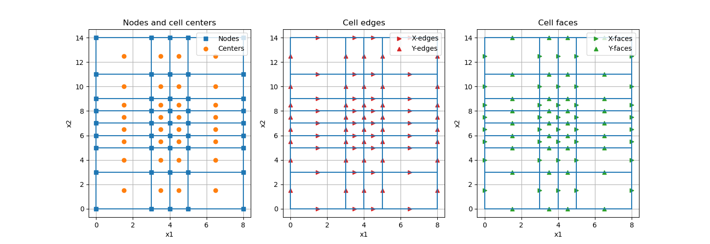
Text(0.5, 1.0, 'Cell faces')

Note that we define X-edges as being edges that lie parallel to the x-axis. And we define X-faces as being faces whose normal lies parallel to the axis. In 3D, the difference between edges and faces is more obvious.