Tree Meshes

Compared to tensor meshes, tree meshes are able to provide higher levels of discretization in certain regions while reducing the total number of cells. Tree meshes belong to the class (TreeMesh). Tree meshes can be defined in 2 or 3 dimensions. Here we demonstrate:

• How to create basic tree meshes in 2D and 3D

• Strategies for local mesh refinement

• How to plot tree meshes

• How to extract properties from tree meshes

To create a tree mesh, we first define the base tensor mesh (a mesh comprised entirely of the smallest cells). Next we choose the level of discretization around certain points or within certain regions. When creating tree meshes, we must remember certain rules:

• The number of base mesh cells in x, y and z must all be powers of 2

• We cannot refine the mesh to create cells smaller than those defining the base mesh

• The range of cell sizes in the tree mesh depends on the number of base mesh cells in x, y and z

Import Packages

Here we import the packages required for this tutorial.

from discretize import TreeMesh
from discretize.utils import mkvc
import matplotlib.pyplot as plt
import numpy as np

# sphinx_gallery_thumbnail_number = 4

Basic Example

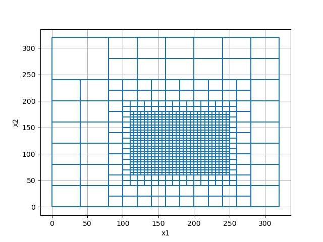
Here we demonstrate the basic two step process for creating a 2D tree mesh (QuadTree mesh). The region of highest discretization if defined within a rectangular box. We use the keyword argument octree_levels to define the rate of cell width increase outside the box.

dh = 5  # minimum cell width (base mesh cell width)
nbc = 64  # number of base mesh cells in x

# Define base mesh (domain and finest discretization)
h = dh * np.ones(nbc)
mesh = TreeMesh([h, h])

# Define corner points for rectangular box
xp, yp = np.meshgrid([120.0, 240.0], [80.0, 160.0])
xy = np.c_[mkvc(xp), mkvc(yp)]  # mkvc creates vectors

# Discretize to finest cell size within rectangular box, with padding in the z direction
# at the finest and second finest levels.
padding = [[0, 2], [0, 2]]
mesh.refine_bounding_box(xy, level=-1, padding_cells_by_level=padding)

mesh.plot_grid(show_it=True)

<Axes: xlabel='x1', ylabel='x2'>

Intermediate Example and Plotting

The widths of the base mesh cells do not need to be the same in x and y. However the number of base mesh cells in x and y each needs to be a power of 2.

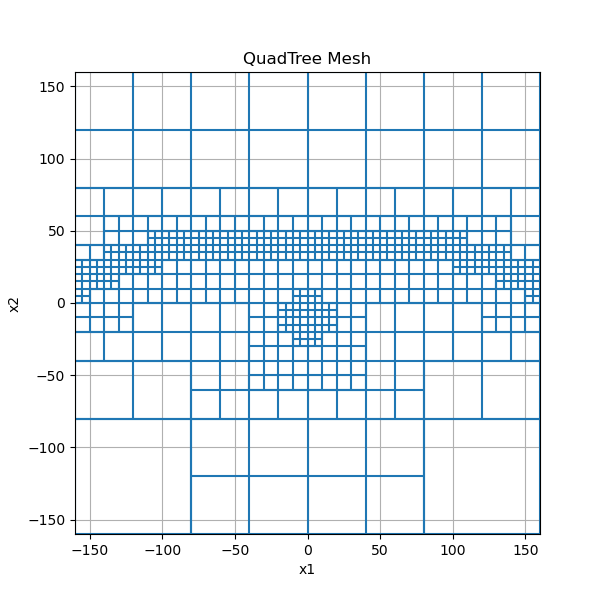
Here we show topography-based mesh refinement and refinement about a set of points. We also show some aspect of customizing plots. We use the keyword argument octree_levels to define the rate of cell width increase relative to our surface and the set of discrete points about which we are refining.

dx = 5  # minimum cell width (base mesh cell width) in x
dy = 5  # minimum cell width (base mesh cell width) in y

x_length = 300.0  # domain width in x
y_length = 300.0  # domain width in y

# Compute number of base mesh cells required in x and y
nbcx = 2 ** int(np.round(np.log(x_length / dx) / np.log(2.0)))
nbcy = 2 ** int(np.round(np.log(y_length / dy) / np.log(2.0)))

# Define the base mesh
hx = [(dx, nbcx)]
hy = [(dy, nbcy)]
mesh = TreeMesh([hx, hy], x0="CC")

# Refine surface topography
xx = mesh.nodes_x
yy = -3 * np.exp((xx**2) / 100**2) + 50.0
pts = np.c_[mkvc(xx), mkvc(yy)]
padding = [[0, 2], [0, 2]]
mesh.refine_surface(pts, padding_cells_by_level=padding, finalize=False)

# Refine mesh near points
xx = np.array([0.0, 10.0, 0.0, -10.0])
yy = np.array([-20.0, -10.0, 0.0, -10])
pts = np.c_[mkvc(xx), mkvc(yy)]
mesh.refine_points(pts, padding_cells_by_level=[2, 2], finalize=False)

mesh.finalize()

# We can apply the plot_grid method and output to a specified axes object
fig = plt.figure(figsize=(6, 6))
ax = fig.add_subplot(111)
mesh.plot_grid(ax=ax)
ax.set_xbound(mesh.x0[0], mesh.x0[0] + np.sum(mesh.h[0]))
ax.set_ybound(mesh.x0[1], mesh.x0[1] + np.sum(mesh.h[1]))
ax.set_title("QuadTree Mesh")

Text(0.5, 1.0, 'QuadTree Mesh')

Extracting Mesh Properties

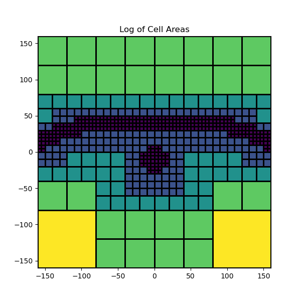
Once the mesh is created, you may want to extract certain properties. Here, we show some properties that can be extracted from a QuadTree mesh.

dx = 5  # minimum cell width (base mesh cell width) in x
dy = 5  # minimum cell width (base mesh cell width) in y

x_length = 300.0  # domain width in x
y_length = 300.0  # domain width in y

# Compute number of base mesh cells required in x and y
nbcx = 2 ** int(np.round(np.log(x_length / dx) / np.log(2.0)))
nbcy = 2 ** int(np.round(np.log(y_length / dy) / np.log(2.0)))

# Define the base mesh
hx = [(dx, nbcx)]
hy = [(dy, nbcy)]
mesh = TreeMesh([hx, hy], x0="CC")

# Refine surface topography
xx = mesh.nodes_x
yy = -3 * np.exp((xx**2) / 100**2) + 50.0
pts = np.c_[mkvc(xx), mkvc(yy)]
padding = [[0, 2], [0, 2]]
mesh.refine_surface(pts, padding_cells_by_level=padding, finalize=False)

# Refine near points
xx = np.array([0.0, 10.0, 0.0, -10.0])
yy = np.array([-20.0, -10.0, 0.0, -10])
pts = np.c_[mkvc(xx), mkvc(yy)]
mesh.refine_points(pts, padding_cells_by_level=[2, 2], finalize=False)

mesh.finalize()

# The bottom west corner
x0 = mesh.x0

# The total number of cells
nC = mesh.nC

# An (nC, 2) array containing the cell-center locations
cc = mesh.gridCC

# A boolean array specifying which cells lie on the boundary
bInd = mesh.cell_boundary_indices

# The cell areas (2D "volume")
s = mesh.cell_volumes

fig = plt.figure(figsize=(6, 6))
ax = fig.add_subplot(111)
mesh.plot_image(np.log10(s), grid=True, ax=ax)
ax.set_xbound(mesh.x0[0], mesh.x0[0] + np.sum(mesh.h[0]))
ax.set_ybound(mesh.x0[1], mesh.x0[1] + np.sum(mesh.h[1]))
ax.set_title("Log of Cell Areas")

Text(0.5, 1.0, 'Log of Cell Areas')

3D Example

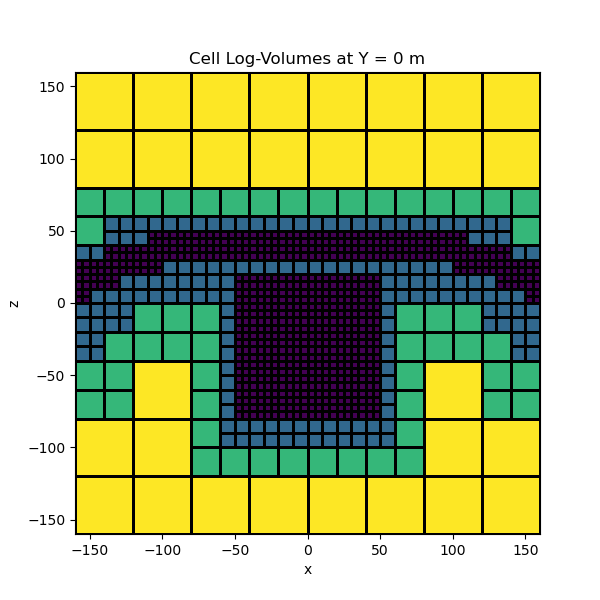
Here we show how the same approach can be used to create and extract properties from a 3D tree mesh.

dx = 5  # minimum cell width (base mesh cell width) in x
dy = 5  # minimum cell width (base mesh cell width) in y
dz = 5  # minimum cell width (base mesh cell width) in z

x_length = 300.0  # domain width in x
y_length = 300.0  # domain width in y
z_length = 300.0  # domain width in y

# Compute number of base mesh cells required in x and y
nbcx = 2 ** int(np.round(np.log(x_length / dx) / np.log(2.0)))
nbcy = 2 ** int(np.round(np.log(y_length / dy) / np.log(2.0)))
nbcz = 2 ** int(np.round(np.log(z_length / dz) / np.log(2.0)))

# Define the base mesh
hx = [(dx, nbcx)]
hy = [(dy, nbcy)]
hz = [(dz, nbcz)]
mesh = TreeMesh([hx, hy, hz], x0="CCC")

# Refine surface topography
[xx, yy] = np.meshgrid(mesh.nodes_x, mesh.nodes_y)
zz = -3 * np.exp((xx**2 + yy**2) / 100**2) + 50.0
pts = np.c_[mkvc(xx), mkvc(yy), mkvc(zz)]
padding = [[0, 0, 2], [0, 0, 2]]
mesh.refine_surface(pts, padding_cells_by_level=padding, finalize=False)

# Refine box
xp, yp, zp = np.meshgrid([-40.0, 40.0], [-40.0, 40.0], [-60.0, 0.0])
xyz = np.c_[mkvc(xp), mkvc(yp), mkvc(zp)]
mesh.refine_bounding_box(xyz, padding_cells_by_level=padding, finalize=False)
mesh.finalize()

# The bottom west corner
x0 = mesh.x0

# The total number of cells
nC = mesh.nC

# An (nC, 3) array containing the cell-center locations
cc = mesh.gridCC

# A boolean array specifying which cells lie on the boundary
bInd = mesh.cell_boundary_indices

# Cell volumes
v = mesh.cell_volumes

fig = plt.figure(figsize=(6, 6))
ax = fig.add_subplot(111)
mesh.plot_slice(np.log10(v), normal="Y", ax=ax, ind=int(mesh.h[1].size / 2), grid=True)
ax.set_title("Cell Log-Volumes at Y = 0 m")

Text(0.5, 1.0, 'Cell Log-Volumes at Y = 0 m')