Slicer demo

The example demonstrates the plot_3d_slicer

• contributed by @prisae

Using the inversion result from the example notebook plot_laguna_del_maule_inversion.ipynb

In the notebook, you have to use %matplotlib notebook.

# %matplotlib notebook
import os
import discretize
import numpy as np
import tarfile
import matplotlib.pyplot as plt
from matplotlib.colors import SymLogNorm

Download and load data

In the following we load the mesh and Lpout that you would get from running the laguna-del-maule inversion notebook.

f = discretize.utils.download(
    "https://storage.googleapis.com/simpeg/laguna_del_maule_slicer.tar.gz",
    overwrite=True,
)
tar = tarfile.open(f, "r")
tar.extractall()
tar.close()

# Load the mesh and model
mesh = discretize.load_mesh(os.path.join("laguna_del_maule_slicer", "mesh.json"))
Lpout = np.load(os.path.join("laguna_del_maule_slicer", "Lpout.npy"))

overwriting /home/vsts/work/1/s/examples/laguna_del_maule_slicer.tar.gz
Downloading https://storage.googleapis.com/simpeg/laguna_del_maule_slicer.tar.gz
   saved to: /home/vsts/work/1/s/examples/laguna_del_maule_slicer.tar.gz
Download completed!

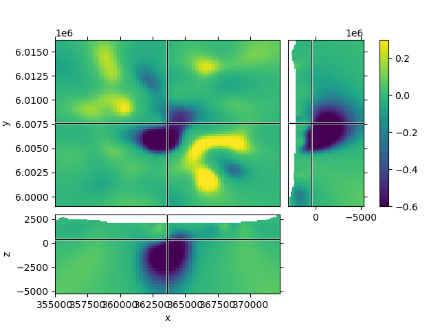
Case 1: Using the intrinsinc functionality

1.1 Default options

mesh.plot_3d_slicer(Lpout)

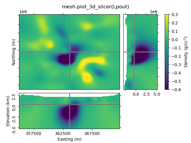
1.2 Create a function to improve plots, labeling after creation

Depending on your data the default option might look a bit odd. The look of the figure can be improved by getting its handle and adjust it.

def beautify(title, fig=None):
    """Beautify the 3D Slicer result."""

    # Get figure handle if not provided
    if fig is None:
        fig = plt.gcf()

    # Get principal figure axes
    axs = fig.get_children()

    # Set figure title
    fig.suptitle(title, y=0.95, va="center")

    # Adjust the y-labels on the first subplot (XY)
    plt.setp(axs[1].yaxis.get_majorticklabels(), rotation=90)
    for label in axs[1].yaxis.get_ticklabels():
        label.set_visible(False)
    for label in axs[1].yaxis.get_ticklabels()[::3]:
        label.set_visible(True)
    axs[1].set_ylabel("Northing (m)")

    # Adjust x- and y-labels on the second subplot (XZ)
    axs[2].set_xticks([357500, 362500, 367500])
    axs[2].set_xlabel("Easting (m)")

    plt.setp(axs[2].yaxis.get_majorticklabels(), rotation=90)
    axs[2].set_yticks([2500, 0, -2500, -5000])
    axs[2].set_yticklabels(["$2.5$", "0.0", "-2.5", "-5.0"])
    axs[2].set_ylabel("Elevation (km)")

    # Adjust x-labels on the third subplot (ZY)
    axs[3].set_xticks([2500, 0, -2500, -5000])
    axs[3].set_xticklabels(["", "0.0", "-2.5", "-5.0"])

    # Adjust colorbar
    axs[4].set_ylabel("Density (g/cc$^3$)")

    # Ensure sufficient margins so nothing is clipped
    plt.subplots_adjust(bottom=0.1, top=0.9, left=0.1, right=0.9)

mesh.plot_3d_slicer(Lpout)
beautify("mesh.plot_3d_slicer(Lpout)")

1.3 Set xslice, yslice, and zslice; transparent region

The 2nd-4th input arguments are the initial x-, y-, and z-slice location (they default to the middle of the volume). The transparency-parameter can be used to define transparent regions.

mesh.plot_3d_slicer(Lpout, 370000, 6002500, -2500, transparent=[[-0.02, 0.1]])
beautify(
    "mesh.plot_3d_slicer("
    "\nLpout, 370000, 6002500, -2500, transparent=[[-0.02, 0.1]])"
)

1.4 Set clim, use pcolor_opts to show grid lines

mesh.plot_3d_slicer(
    Lpout, clim=[-0.4, 0.2], pcolor_opts={"edgecolor": "k", "linewidth": 0.1}
)
beautify(
    "mesh.plot_3d_slicer(\nLpout, clim=[-0.4, 0.2], "
    "pcolor_opts={'edgecolor': 'k', 'linewidth': 0.1})"
)

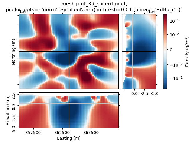
1.5 Use pcolor_opts to set SymLogNorm, and another cmap

mesh.plot_3d_slicer(
    Lpout, pcolor_opts={"norm": SymLogNorm(linthresh=0.01), "cmap": "RdBu_r"}
)
beautify(
    "mesh.plot_3d_slicer(Lpout,"
    "\npcolor_opts={'norm': SymLogNorm(linthresh=0.01),'cmap': 'RdBu_r'})`"
)

1.6 Use aspect and grid

By default, aspect='auto' and grid=[2, 2, 1]. This means that the figure is on a 3x3 grid, where the xy-slice occupies 2x2 cells of the subplot-grid, xz-slice 2x1, and the zy-silce 1x2. So the grid=[x, y, z]-parameter takes the number of cells for x, y, and z-dimension.

grid can be used to improve the probable weired subplot-arrangement if aspect is anything else than auto. However, if you zoom then it won’t help. Expect the unexpected.

mesh.plot_3d_slicer(Lpout, aspect=["equal", 1.5], grid=[4, 4, 3])
beautify("mesh.plot_3d_slicer(Lpout, aspect=['equal', 1.5], grid=[4, 4, 3])")

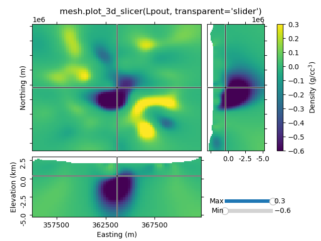
1.7 Transparency-slider

Setting the transparent-parameter to ‘slider’ will create interactive sliders to change which range of values of the data is visible.

mesh.plot_3d_slicer(Lpout, transparent="slider")
beautify("mesh.plot_3d_slicer(Lpout, transparent='slider')")

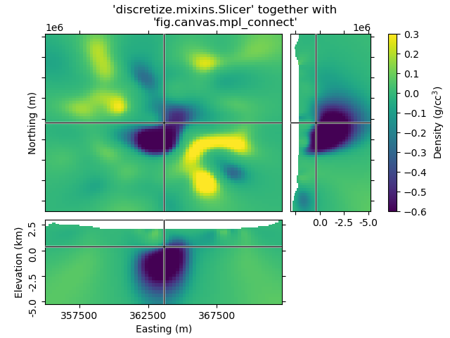
Case 2: Just using the Slicer class

This way you get the figure-handle, and can do further stuff with the figure.

# You have to initialize a figure
fig = plt.figure()

# Then you have to get the tracker from the Slicer
tracker = discretize.mixins.Slicer(mesh, Lpout)

# Finally you have to connect the tracker to the figure
fig.canvas.mpl_connect("scroll_event", tracker.onscroll)

# Run it through beautify
beautify("'discretize.mixins.Slicer' together with\n'fig.canvas.mpl_connect'", fig)

plt.show()