Note
Go to the end to download the full example code.
3D Visualization with PyVista#
The example demonstrates the how to use the VTK interface via the pyvista library . To run this example, you will need to install pyvista .
contributed by @banesullivan
Using the inversion result from the example notebook plot_laguna_del_maule_inversion.ipynb
# sphinx_gallery_thumbnail_number = 2
import discretize
import pyvista as pv
import numpy as np
import pooch

# Set a documentation friendly plotting theme
pv.set_plot_theme("document")

print("PyVista Version: {}".format(pv.__version__))
PyVista Version: 0.48.4
Download and load data#
In the following we load the mesh and Lpout that you would
get from running the laguna-del-maule inversion notebook as well as some of
the raw data for the topography surface and gravity observations.
# Download Topography and Observed gravity data
data_url = "https://storage.googleapis.com/simpeg/Chile_GRAV_4_Miller/Chile_GRAV_4_Miller.tar.gz"
downloaded_items = pooch.retrieve(
    data_url,
    known_hash="28022bf8802eeb4892cac6c3efd1eb4275c84003a6723c047fe5e1738a66ea04",
    processor=pooch.Untar(),
)
data_path = next(filter(lambda f: f.endswith("LdM_grav_obs.grv"), downloaded_items))
topo_path = next(filter(lambda f: f.endswith("LdM_topo.topo"), downloaded_items))

model_url = "https://storage.googleapis.com/simpeg/laguna_del_maule_slicer.tar.gz"
downloaded_items = pooch.retrieve(
    model_url,
    known_hash="107293bfdeb77b314f4cb451a24c2c93a55aae40da28f43cf3c075d71acfb957",
    processor=pooch.Untar(),
)
mesh_path = next(filter(lambda f: f.endswith("mesh.json"), downloaded_items))
model_path = next(filter(lambda f: f.endswith("Lpout.npy"), downloaded_items))

# # Load the mesh/data
mesh = discretize.load_mesh(mesh_path)
models = {"Lpout": np.load(model_path)}
Create PyVista data objects#
Here we start making PyVista data objects of all the spatially referenced data.
# Get the PyVista dataset of the inverted model
dataset = mesh.to_vtk(models)
dataset.set_active_scalars("Lpout")
(<FieldAssociation.CELL: 1>, pyvista_ndarray([0.02552159, 0.02554211, 0.02568049, ...,        nan,
                        nan,        nan], shape=(190440,)))
# Load topography points from text file as XYZ numpy array
topo_pts = np.loadtxt(topo_path, skiprows=1)
# Create the topography points and apply an elevation filter
topo = pv.PolyData(topo_pts).delaunay_2d().elevation()
# Load the gravity data from text file as XYZ+attributes numpy array
grav_data = np.loadtxt(data_path, skiprows=1)
print("gravity file shape: ", grav_data.shape)
# Use the points to create PolyData
grav = pv.PolyData(grav_data[:, 0:3])
# Add the data arrays
grav.point_data["comp-1"] = grav_data[:, 3]
grav.point_data["comp-2"] = grav_data[:, 4]
grav.set_active_scalars("comp-1")
gravity file shape:  (191, 5)

(<FieldAssociation.POINT: 0>, pyvista_ndarray([-1.15534e+01, -1.44465e+01, -5.33190e+00, -1.63014e+01,
                 -1.30721e+01, -1.39600e-01,  5.68720e+00, -7.10900e-01,
                  4.71980e+00,  1.23900e+00,  3.68730e+00, -5.31380e+00,
                  4.14140e+00, -3.58090e+00,  3.94350e+00,  4.07840e+00,
                 -1.14430e+00,  3.99480e+00,  5.58800e-01, -1.40378e+01,
                 -1.43858e+01, -1.63174e+01, -1.16554e+01, -2.87140e+00,
                 -9.56420e+00, -2.25410e+00, -4.58700e-01, -5.24410e+00,
                  4.90410e+00,  5.52340e+00,  3.87690e+00,  4.02540e+00,
                  3.81050e+00,  2.83610e+00,  2.56460e+00, -1.63680e+00,
                 -4.29360e+00, -5.44530e+00, -3.38050e+00, -3.28940e+00,
                 -1.83590e+00, -8.48700e-01, -1.09720e+00, -1.92030e+00,
                 -8.58400e-01,  9.17100e-01,  2.08710e+00,  3.63410e+00,
                  3.87850e+00,  4.20830e+00,  3.76590e+00,  4.37010e+00,
                  4.97830e+00,  5.47840e+00,  4.20080e+00,  4.53510e+00,
                  3.87420e+00,  3.80150e+00,  3.70450e+00,  4.18960e+00,
                  4.14460e+00,  3.69240e+00,  2.99500e+00,  2.57130e+00,
                  2.82980e+00,  4.18930e+00,  2.37200e+00,  2.24040e+00,
                 -1.57320e+00, -2.95570e+00, -6.11860e+00, -8.62850e+00,
                  4.23130e+00,  3.87100e+00,  4.25970e+00,  3.98770e+00,
                  3.07480e+00,  2.33480e+00, -1.16109e+01, -9.84730e+00,
                 -5.55460e+00, -9.33400e-01, -7.04800e-01, -2.49900e-01,
                 -1.01720e+00,  1.10040e+00,  7.12600e-01,  5.52700e-02,
                 -4.48000e-02, -6.12000e-01, -2.54110e+00, -5.06770e+00,
                 -1.33736e+01,  4.70080e+00,  2.96350e+00,  1.79560e+00,
                  1.23870e+00,  4.76700e-01,  3.94200e-01,  4.63400e-01,
                  1.67910e+00, -2.09600e-01, -1.03530e+00, -2.36800e-01,
                 -3.75900e-01,  1.89900e+00,  3.70720e+00,  5.07700e+00,
                  6.06070e+00,  4.37360e+00,  4.37840e+00,  2.24920e+00,
                  2.81660e+00,  5.34190e+00,  5.86920e+00,  4.18790e+00,
                  3.95290e+00,  8.15200e-01, -1.27156e+01, -1.43970e+01,
                 -1.74116e+01, -1.86309e+01, -1.81361e+01,  4.94820e+00,
                  3.93680e+00,  1.32440e+00, -3.41200e-01,  1.65010e+00,
                 -1.22760e+00, -1.81560e+00, -3.28520e+00, -3.09490e+00,
                 -4.19520e+00, -3.48290e+00, -3.78440e+00, -3.26540e+00,
                 -3.08930e+00, -3.90630e+00, -4.93810e+00, -7.21930e+00,
                 -5.10450e+00, -9.73700e-01, -9.08700e-01,  2.24600e-01,
                 -8.98800e-01, -4.72800e-01, -1.19300e-01, -1.83000e-02,
                 -1.00700e+00, -8.17600e-01, -1.45390e+00, -1.59900e-01,
                 -8.91000e-02, -1.34800e+00,  5.03900e-01, -6.82900e-01,
                 -1.38463e+01, -1.56983e+01, -1.27892e+01, -1.24353e+01,
                  5.16970e+00,  7.08610e+00,  8.82880e+00,  9.56390e+00,
                  9.91700e+00,  9.10020e+00,  7.98270e+00,  7.49300e+00,
                 -3.28730e+00,  9.36000e-02,  3.46120e+00,  2.97870e+00,
                  1.67290e+00,  2.43910e+00, -2.80870e+00, -2.44900e+00,
                 -9.97900e-01, -1.97800e-01, -1.08000e-01, -2.63600e-01,
                  8.78000e-02,  4.40860e+00, -6.57400e-01,  8.15900e-01,
                  7.45070e+00,  7.13330e+00,  1.13950e+00, -2.55000e-02,
                  1.07700e+00, -2.95130e+00,  1.58060e+00]))
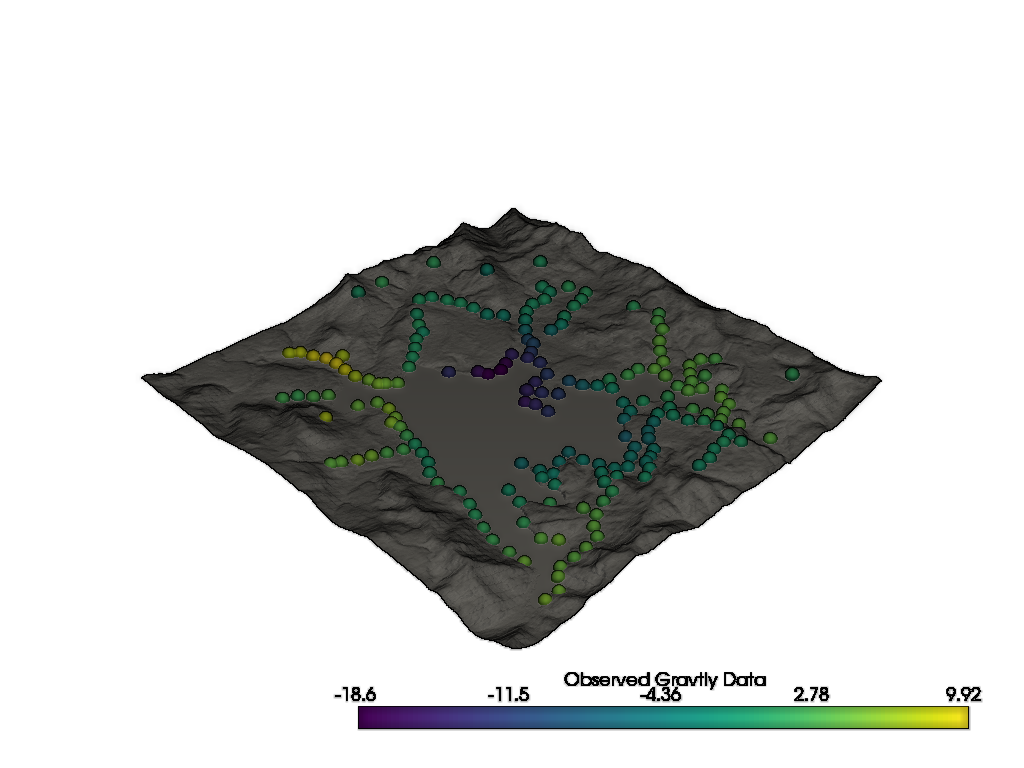
Plot the topographic surface and the gravity data
p = pv.Plotter()
p.add_mesh(topo, color="grey")
p.add_mesh(
    grav,
    point_size=15,
    render_points_as_spheres=True,
    scalar_bar_args={"title": "Observed Gravtiy Data"},
)
# Use a non-phot-realistic shading technique to show topographic relief
p.enable_eye_dome_lighting()
p.show(window_size=[1024, 768])
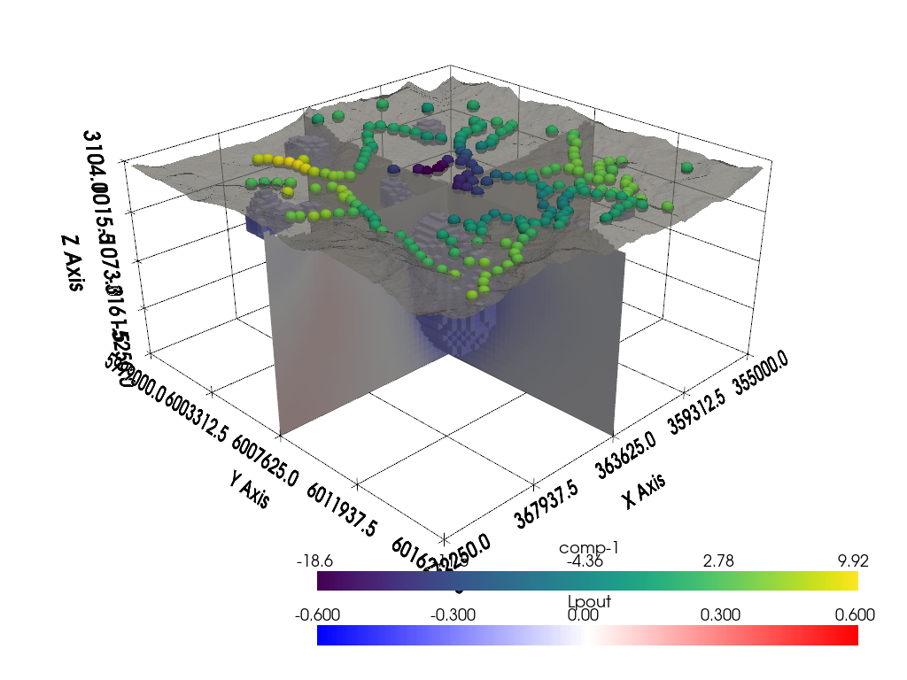
Visualize Using PyVista#
Here we visualize all the data in 3D!
# Create display parameters for inverted model
dparams = dict(
    show_edges=False,
    cmap="bwr",
    clim=[-0.6, 0.6],
)

# Apply a threshold filter to remove topography
#  no arguments will remove the NaN values
dataset_t = dataset.threshold()

# Extract volumetric threshold
threshed = dataset_t.threshold(-0.2, invert=True)

# Create the rendering scene
p = pv.Plotter()
# add a grid axes
p.show_grid()

# Add spatially referenced data to the scene
p.add_mesh(dataset_t.slice("x"), **dparams)
p.add_mesh(dataset_t.slice("y"), **dparams)
p.add_mesh(threshed, **dparams)
p.add_mesh(
    topo,
    opacity=0.75,
    color="grey",
    # cmap='gist_earth', clim=[1.7e+03, 3.104e+03],
)
p.add_mesh(grav, cmap="viridis", point_size=15, render_points_as_spheres=True)

# Here is a nice camera position we manually found:
cpos = [
    (395020.7332989303, 6039949.0452080015, 20387.583125699253),
    (364528.3152860675, 6008839.363092581, -3776.318305935185),
    (-0.3423732500124074, -0.34364514928896667, 0.8744647328772646),
]
p.camera_position = cpos


# Render the scene!
p.show(window_size=[1024, 768])
Total running time of the script: (0 minutes 14.141 seconds)