Note

Go to the end to download the full example code.

Nodal Dirichlet Poisson solution#

In this example, we demonstrate how to solve a Poisson equation where the solution lives on nodes, and we want to impose Dirichlet conditions on the boundary.

Solve a nodal Poisson’s equation with Dirichlet boundary conditions#

The PDE we want to solve is Poisson’s equation with a variable conductivity, where we know the value of the solution on the boundary.

\begin{array}{r} - \nabla \cdot σ \nabla u = f \\ u = q on \partial Ω \end{array}

We express this in a weak form, where we multiply by an arbitrary test function and integrate over the volume:

⟨ w, \nabla \cdot - σ \nabla u ⟩ = ⟨ w, f ⟩

The left hand side can be changed to avoid taking the divergence of $- σ \nabla u$ using a higher dimension integration by parts, instead transfering the differentiability to $w$ .

⟨ \nabla w, σ \nabla u ⟩ - \int_{\partial Ω} w (σ \nabla u) \cdot \hat{n} d A = ⟨ w, f ⟩

We are interested in solving this where $u$ , $f$ , and $w$ are defined on cell nodes, $σ$ is defined on cell centers. Also of note is that in the finite volume formulation we approximate the solution as integrals of averages over each cell and the test functions and basis functions are piecewise constant. Thus our discrete form goes to:

w^{T} G^{T} M_{e, σ} G u - w_{b}^{T} b_{c} = w^{T} M_{n} f

with $b_{c}$ representing the boundary condition on $(σ \nabla u) \cdot \hat{n}$ . Where $G$ is a nodal gradient operator that estimates the gradient at the edge centers, $M_{e, σ}$ represents the inner product of vectors that live on mesh edges taken with respect to $σ$ , and $M_{n}$ is correspondingly the inner product operator for scalars that live on mesh nodes.

Taking care of the boundaries#

Set $u_{b}$ , and $w_{b}$ as the values of $u$ and $w$ on the boundary, and $u_{f}$ and $w_{f}$ the values of $u$ and $w$ on the interior. We have that

\begin{array}{r} w = P_{f} w_{f} + P_{b} w_{b} \\ u = P_{f} u_{f} + P_{b} u_{b} \end{array}

Where $P_{b}$ and $P_{f}$ are the matrices which project the values on the boundary and free interior nodes, respectively, to all of the nodes.

There is much freedom in what we choose to be our test functions, and to avoid the integral on the boundary without assuming a value for $(σ \nabla u) \cdot \hat{n}$ , we set that our test functions are zero on the boundary, $w_{b} = 0$

Thus the full system is

w_{f}^{T} P_{f}^{T} G^{T} M_{e, σ} G (P_{f} u_{f} + P_{b} u_{b}) = w_{f}^{T} P_{f}^{T} M_{n} f

Our final system of equations#

The above scalar equality must be true for all vectors $w$ , thus the vectors are also equal:

P_{f}^{T} G^{T} M_{e, σ} G (P_{f} u_{f} + P_{b} u_{b}) = P_{f}^{T} M_{n} f

We then collect the unknowns $u_{f}$ on the left hand side, and move everything else to the right.

P_{f}^{T} G^{T} M_{e, σ} G P_{f} u_{f} = P_{f}^{T} M_{n} f - P_{f}^{T} G^{T} M_{e, σ} G P_{b} u_{b}

Now lets actually code this solution up using these matrices!

import numpy as np
import discretize
import matplotlib.pyplot as plt
import scipy.sparse as sp
from discretize import tests

import sympy
import sympy.vector as spv
from sympy.utilities.lambdify import lambdify

Our PDE#

We are going to setup a simple two-dimensional problem which we will solve on a TensorMesh. We want to test the accuracy of our discretization scheme for the problem (it should be second order accurate). Thus we define a known solution $u$ and property model $σ$ . Then we use sympy to do all the derivatives for us to determine the correct forcing function.

\begin{array}{r} u = \sin (x) \cos (y) e^{x + y} \\ σ = \cos (x) \sin (y) \end{array}

C = spv.CoordSys3D("u")

u = sympy.sin(C.x) * sympy.cos(C.y) * sympy.exp(C.x + C.y)
sig = sympy.cos(C.x) * sympy.sin(C.y)

f = -spv.divergence(sig * spv.gradient(u))

# lambdify the functions so we can evalute them at any requested location
u_func = lambdify([C.x, C.y], u)
sig_func = lambdify([C.x, C.y], sig)
f_func = lambdify([C.x, C.y], f)
print(f)

-(-exp(u.x + u.y)*sin(u.x)*sin(u.y) + exp(u.x + u.y)*sin(u.x)*cos(u.y))*cos(u.x)*cos(u.y) + (exp(u.x + u.y)*sin(u.x)*cos(u.y) + exp(u.x + u.y)*cos(u.x)*cos(u.y))*sin(u.x)*sin(u.y) + 2*exp(u.x + u.y)*sin(u.x)*sin(u.y)**2*cos(u.x) - 2*exp(u.x + u.y)*sin(u.y)*cos(u.x)**2*cos(u.y)

Next we are going to solve our PDE! We encapsulate the code into a function that returns the error and discretization size, so we can use discretize’s testing utilities to perform an order test for us.

def get_error(n_cells, plot_it=False):
    # Create a mesh with a certain number of cells on the [0, 1] square
    mesh = discretize.TensorMesh([n_cells, n_cells])
    h = mesh.nodes_x[1] - mesh.nodes_x[0]

    # evaluate our boundary conditions, the sigma model, and
    # the forcing function.
    u_b = u_func(*mesh.boundary_nodes.T)
    sig_cc = sig_func(*mesh.cell_centers.T)
    f_n = f_func(*mesh.nodes.T)

    # Get the finite volume operators for the mesh
    G = mesh.nodal_gradient
    M_e_sigma = mesh.get_edge_inner_product(sig_cc)
    M_n = sp.diags(mesh.average_node_to_cell.T @ mesh.cell_volumes)

    # Determin which mesh nodes are on the boundary, and which are interior
    is_boundary = np.zeros(mesh.n_nodes, dtype=bool)
    is_boundary[mesh.project_node_to_boundary_node.indices] = True

    # construct the projection matrices
    P_b = sp.eye(mesh.n_nodes, format="csc")[:, is_boundary]
    P_f = sp.eye(mesh.n_nodes, format="csc")[:, ~is_boundary]

    # Assemble the solution matrix and rhs.
    A = P_f.T @ G.T @ M_e_sigma @ G @ P_f
    rhs = P_f.T @ M_n @ f_n - P_f.T @ G.T @ M_e_sigma @ G @ P_b @ u_b

    # Solve for the value of u on the free nodes, then project
    # with the boundary conditions to obtain the solution on
    # all nodes.
    u_f = sp.linalg.spsolve(A, rhs)
    u_sol = P_f @ u_f + P_b @ u_b

    # Since we know the true solution we can check the error
    # which we expect to be second order accurate.
    u_true = u_func(*mesh.nodes.T)
    err = np.linalg.norm(u_sol - u_true, ord=np.inf)

    # Add some codes for us to use this function to plot the solution.
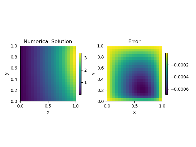
    if plot_it:
        ax = plt.subplot(121)
        (im,) = mesh.plot_image(u_sol, v_type="N", ax=ax)
        ax.set_title("Numerical Solution")
        ax.set_aspect("equal")
        plt.colorbar(im, shrink=0.3)

        ax = plt.subplot(122)
        (im,) = mesh.plot_image(u_sol - u_true, v_type="N", ax=ax)
        ax.set_title("Error")
        ax.set_aspect("equal")
        plt.colorbar(im, shrink=0.3)
        plt.tight_layout()
        plt.show()
    else:
        return err, h

Lets look at the solution itself!

get_error(20, plot_it=True)

Order Testing#

To verify our discretization strategy we will use the above function to perform a convergence test. We make use of the assert_expected_order function to print out a convergence table. This will raise an error if our convergence is not what we expect.

tests.assert_expected_order(get_error, [10, 20, 30, 40, 50])

_______________________________________________________
  nc  |    h    |    error    | e(i-1)/e(i) |  order
~~~~~~|~~~~~~~~~|~~~~~~~~~~~~~|~~~~~~~~~~~~~|~~~~~~~~~~
  10  |1.00e-01 |  2.558e-03  |             |
  20  |5.00e-02 |  6.903e-04  |   3.7055    |  1.8897
  30  |3.33e-02 |  3.159e-04  |   2.1850    |  1.9277
  40  |2.50e-02 |  1.811e-04  |   1.7443    |  1.9340
  50  |2.00e-02 |  1.174e-04  |   1.5421    |  1.9411
-------------------------------------------------------
Not just a pretty face Vsts

[np.float64(1.8896629662199587), np.float64(1.9276904648779223), np.float64(1.9340112284566402), np.float64(1.9410749331527082)]

Total running time of the script: (0 minutes 0.567 seconds)

Gallery generated by Sphinx-Gallery