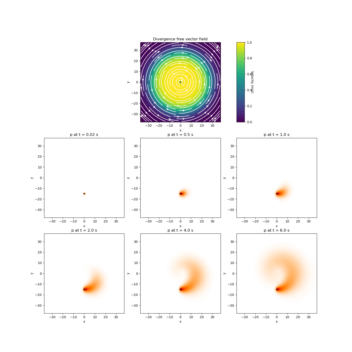
Advection-Diffusion Equation

Here we use the discretize package to model the advection-diffusion equation. The goal of this tutorial is to demonstrate:

• How to solve time-dependent PDEs

• How to apply Neumann boundary conditions

• Strategies for applying finite volume to 2nd order PDEs

Derivation

If we assume the fluid is incompressible (\(\nabla \cdot \mathbf{u} = 0\)), the advection-diffusion equation with Neumann boundary conditions is given by:

\[\begin{split}p_t = \nabla \cdot \alpha \nabla p - \mathbf{u} \cdot \nabla p + s \\ \textrm{s.t.} \;\;\; \frac{\partial p}{\partial n} \Bigg |_{\partial \Omega} = 0\end{split}\]

where \(p\) is the unknown variable, \(\alpha\) defines the diffusivity within the domain, \(\mathbf{u}\) is the velocity field, and \(s\) is the source term. We will consider the case where there is a single point source within our domain. Thus:

\[s = s_0 \delta ( \mathbf{r} )\]

where \(s_0\) is a constant. To solve this problem numerically, we re-express the advection-diffusion equation as a set of first order PDEs:

\[\begin{split}\; \; p_t = \nabla \cdot \mathbf{j} - \mathbf{u} \cdot \mathbf{w} + s \;\;\; (1)\\ \; \; \mathbf{w} = \nabla p \;\;\; (2) \\ \; \; \alpha^{-1} \mathbf{j} = \mathbf{w} \;\;\; (3)\end{split}\]

We then apply the weak formulation; that is, we take the inner product of each equation with an appropriate test function.

Expression 1:

Let \(\psi\) be a scalar test function. By taking the inner product with expression (1) we obtain:

\[\int_\Omega \psi \, p_t \, dv = \int_\Omega \psi \, (\nabla \cdot \mathbf{j}) \, dv - \int_\Omega \psi \, \big ( \mathbf{u} \cdot \mathbf{w} \big ) \, dv + s_0 \int_\Omega \psi \, \delta (\mathbf{r}) \, dv\]

The source term is a volume integral containing the Dirac delta function, thus:

\[s_0 \int_\Omega \psi \, \delta (\mathbf{r}) \, dv \approx \mathbf{\psi^T \, q}\]

where \(q=s_0\) for the cell containing the point source and zero everywhere else. By evaluating the inner products according to the finite volume approach we obtain:

\[\mathbf{\psi^T M_c p_t} = \mathbf{\psi^T M_c D \, j} - \mathbf{\psi^T M_c A_{fc}} \, \textrm{diag} ( \mathbf{u} ) \mathbf{w} + \mathbf{\psi^T q}\]

where \(\mathbf{\psi}\), \(\mathbf{p}\) and \(\mathbf{p_t}\) live at cell centers and \(\mathbf{j}\), \(\mathbf{u}\) and \(\mathbf{w}\) live on cell faces. \(\mathbf{D}\) is a discrete divergence operator. \(\mathbf{M_c}\) is the cell center inner product matrix. \(\mathbf{A_{fc}}\) takes the dot product of \(\mathbf{u}\) and \(\mathbf{w}\), projects it to cell centers and sums the contributions by each Cartesian component.

Expression 2:

Let \(\mathbf{f}\) be a vector test function. By taking the inner product with expression (2) we obtain:

\[\int_\Omega \mathbf{f \cdot w} \, dv = \int_\Omega \mathbf{f \cdot \nabla}p \, dv\]

If we use the identity \(\phi \nabla \cdot \mathbf{a} = \nabla \cdot (\phi \mathbf{a}) - \mathbf{a} \cdot (\nabla \phi )\) and apply the divergence theorem we obtain:

\[\int_\Omega \mathbf{f \cdot w} \, dv = \int_{\partial \Omega} \mathbf{n \, \cdot} \, p \mathbf{f} \, da - \int_{\Omega} p \cdot \nabla \mathbf{f} \, dv\]

If we assume that \(f=0\) on the boundary, we can eliminate the surface integral. By evaluating the inner products in the weak formulation according to the finite volume approach we obtain:

\[\mathbf{f^T M_f w} = - \mathbf{f^T D^T M_c}p\]

where \(\mathbf{f}\) lives at cell faces and \(\mathbf{M_f}\) is the face inner product matrix.

Expression 3:

Let \(\mathbf{f}\) be a vector test function. By taking the inner product with expression (3) we obtain:

\[\int_\Omega \mathbf{f} \cdot \alpha^{-1} \mathbf{j} \, dv = \int_\Omega \mathbf{f} \cdot \mathbf{w} \, dv\]

By evaluating the inner products according to the finite volume approach we obtain:

\[\mathbf{f^T M_\alpha \, j} = \mathbf{f^T M_f \, w}\]

where \(\mathbf{M_\alpha}\) is a face inner product matrix that depends on the inverse of the diffusivity.

Final Numerical System:

By combining the set of discrete expressions and letting \(\mathbf{s} = \mathbf{M_c^{-1} q}\), we obtain:

\[\mathbf{p_t} = - \mathbf{D M_\alpha^{-1} \, D^T \, M_c} \, p + \mathbf{A_{fc}} \, \textrm{diag} ( \mathbf{u} ) \mathbf{M_f^{-1} D^T \, M_c} p + \mathbf{s}\]

Since the Neumann boundary condition is being used for the variable \(p\), the transpose of the divergence operator is the negative of the gradient operator with Neumann boundary conditions; e.g. \(\mathbf{D^T = -G}\). Thus:

\[\mathbf{p_t} = - \mathbf{M} \mathbf{p} + \mathbf{s}\]

where

\[\mathbf{M} = - \mathbf{D M_\alpha^{-1} \, G \, M_c} \, p + \mathbf{A_{fc}} \, \textrm{diag} ( \mathbf{u} ) \mathbf{M_f^{-1} G \, M_c} p\]

For the example, we will discretize in time using backward Euler. This results in the following system which must be solve at every time step \(k\). Where \(\Delta t\) is the step size:

\[\big [ \mathbf{I} + \Delta t \, \mathbf{M} \big ] \mathbf{p}^{k+1} = \mathbf{p}^k + \Delta t \, \mathbf{s}\]

Import Packages

Here we import the packages required for this tutorial.

from discretize import TensorMesh
from pymatsolver import SolverLU
import matplotlib.pyplot as plt
import matplotlib as mpl
import numpy as np
from discretize.utils import sdiag, mkvc

Solving the Problem

# Create a tensor mesh
h = np.ones(75)
mesh = TensorMesh([h, h], "CC")

# Define a divergence free vector field on faces
faces_x = mesh.gridFx
faces_y = mesh.gridFy

r_x = np.sqrt(np.sum(faces_x**2, axis=1))
r_y = np.sqrt(np.sum(faces_y**2, axis=1))

ux = 0.5 * (-faces_x[:, 1] / r_x) * (1 + np.tanh(0.15 * (28.0 - r_x)))
uy = 0.5 * (faces_y[:, 0] / r_y) * (1 + np.tanh(0.15 * (28.0 - r_y)))

u = 10.0 * np.r_[ux, uy]  # Maximum velocity is 10 m/s

# Define vector q where s0 = 1 in our analytic source term
xycc = mesh.gridCC
k = (xycc[:, 0] == 0) & (xycc[:, 1] == -15)  # source at (0, -15)

q = np.zeros(mesh.nC)
q[k] = 1

# Define diffusivity within each cell
a = mkvc(8.0 * np.ones(mesh.nC))

# Define the matrix M
Afc = mesh.dim * mesh.aveF2CC  # modified averaging operator to sum dot product
Mf_inv = mesh.get_face_inner_product(invert_matrix=True)
Mc = sdiag(mesh.cell_volumes)
Mc_inv = sdiag(1 / mesh.cell_volumes)
Mf_alpha_inv = mesh.get_face_inner_product(a, invert_model=True, invert_matrix=True)

mesh.set_cell_gradient_BC(["neumann", "neumann"])  # Set Neumann BC
G = mesh.cell_gradient
D = mesh.face_divergence

M = -D * Mf_alpha_inv * G * Mc + Afc * sdiag(u) * Mf_inv * G * Mc


# Set time stepping, initial conditions and final matricies
dt = 0.02  # Step width
p = np.zeros(mesh.nC)  # Initial conditions p(t=0)=0

I = sdiag(np.ones(mesh.nC))  # Identity matrix
B = I + dt * M
s = Mc_inv * q

Binv = SolverLU(B)


# Plot the vector field
fig = plt.figure(figsize=(15, 15))
ax = 9 * [None]

ax[0] = fig.add_subplot(332)
mesh.plot_image(
    u,
    ax=ax[0],
    v_type="F",
    view="vec",
    stream_opts={"color": "w", "density": 1.0},
    clim=[0.0, 10.0],
)
ax[0].set_title("Divergence free vector field")

ax[1] = fig.add_subplot(333)
ax[1].set_aspect(10, anchor="W")
cbar = mpl.colorbar.ColorbarBase(ax[1], orientation="vertical")
cbar.set_label("Velocity (m/s)", rotation=270, labelpad=5)

# Perform backward Euler and plot

n = 3

for ii in range(300):
    p = Binv * (p + s)

    if ii + 1 in (1, 25, 50, 100, 200, 300):
        ax[n] = fig.add_subplot(3, 3, n + 1)
        mesh.plot_image(p, v_type="CC", ax=ax[n], pcolor_opts={"cmap": "gist_heat_r"})
        title_str = "p at t = " + str((ii + 1) * dt) + " s"
        ax[n].set_title(title_str)
        n = n + 1