Gauss’ Law of Electrostatics

Here we use the discretize package to solve for the electric potential (\(\phi\)) and electric fields (\(\mathbf{e}\)) in 2D that result from a static charge distribution. Starting with Gauss’ law and Faraday’s law:

\[\begin{split}&\nabla \cdot \mathbf{E} = \frac{\rho}{\epsilon_0} \\ &\nabla \times \mathbf{E} = \mathbf{0} \;\;\; \Rightarrow \;\;\; \mathbf{E} = -\nabla \phi \\ &\textrm{s.t.} \;\;\; \phi \Big |_{\partial \Omega} = 0\end{split}\]

where \(\sigma\) is the charge density and \(\epsilon_0\) is the permittivity of free space. We will consider the case where there is both a positive and a negative charge of equal magnitude within our domain. Thus:

\[\rho = \rho_0 \big [ \delta ( \mathbf{r_+}) - \delta (\mathbf{r_-} ) \big ]\]

To solve this problem numerically, we use the weak formulation; that is, we take the inner product of each equation with an appropriate test function. Where \(\psi\) is a scalar test function and \(\mathbf{f}\) is a vector test function:

\[\begin{split}\int_\Omega \psi (\nabla \cdot \mathbf{E}) dV = \frac{1}{\epsilon_0} \int_\Omega \psi \rho dV \\ \int_\Omega \mathbf{f \cdot E} \, dV = - \int_\Omega \mathbf{f} \cdot (\nabla \phi ) dV\end{split}\]

In the case of Gauss’ law, we have a volume integral containing the Dirac delta function, thus:

\[\int_\Omega \psi (\nabla \cdot \mathbf{E}) dV = \frac{1}{\epsilon_0} \psi \, q\]

where \(q\) represents an integrated charge density. By applying the finite volume approach to this expression we obtain:

\[\mathbf{\psi^T M_c D e} = \frac{1}{\epsilon_0} \mathbf{\psi^T q}\]

where \(\mathbf{q}\) denotes the total enclosed charge for each cell. Thus \(\mathbf{q_i}=\rho_0\) for the cell containing the positive charge and \(\mathbf{q_i}=-\rho_0\) for the cell containing the negative charge. It is zero for every other cell.

\(\mathbf{\psi}\) and \(\mathbf{q}\) live at cell centers and \(\mathbf{e}\) lives on cell faces. \(\mathbf{D}\) is the discrete divergence operator. \(\mathbf{M_c}\) is an inner product matrix for cell centered quantities.

For the second weak form equation, we make use of the divergence theorem as follows:

\[\begin{split}\int_\Omega \mathbf{f \cdot E} \, dV &= - \int_\Omega \mathbf{f} \cdot (\nabla \phi ) dV \\ & = - \frac{1}{\epsilon_0} \int_\Omega \nabla \cdot (\mathbf{f} \phi ) dV + \frac{1}{\epsilon_0} \int_\Omega ( \nabla \cdot \mathbf{f} ) \phi \, dV \\ & = - \frac{1}{\epsilon_0} \int_{\partial \Omega} \mathbf{n} \cdot (\mathbf{f} \phi ) da + \frac{1}{\epsilon_0} \int_\Omega ( \nabla \cdot \mathbf{f} ) \phi \, dV \\ & = 0 + \frac{1}{\epsilon_0} \int_\Omega ( \nabla \cdot \mathbf{f} ) \phi \, dV\end{split}\]

where the surface integral is zero due to the boundary conditions we imposed. Evaluating this expression according to the finite volume approach we obtain:

\[\mathbf{f^T M_f e} = \mathbf{f^T D^T M_c \phi}\]

where \(\mathbf{f}\) lives on cell faces and \(\mathbf{M_f}\) is the inner product matrix for quantities that live on cell faces. By canceling terms and combining the set of discrete equations we obtain:

\[\big [ \mathbf{M_c D M_f^{-1} D^T M_c} \big ] \mathbf{\phi} = \frac{1}{\epsilon_0} \mathbf{q}\]

from which we can solve for \(\mathbf{\phi}\). The electric field can be obtained by computing:

\[\mathbf{e} = \mathbf{M_f^{-1} D^T M_c \phi}\]

Import Packages

Here we import the packages required for this tutorial.

from discretize import TensorMesh
from pymatsolver import SolverLU
import matplotlib.pyplot as plt
import numpy as np
from discretize.utils import sdiag

Solving the Problem

# Create a tensor mesh
h = np.ones(75)
mesh = TensorMesh([h, h], "CC")

# Create system
DIV = mesh.face_divergence  # Faces to cell centers divergence
Mf_inv = mesh.get_face_inner_product(invert_matrix=True)
Mc = sdiag(mesh.cell_volumes)
A = Mc * DIV * Mf_inv * DIV.T * Mc

# Define RHS (charge distributions at cell centers)
xycc = mesh.gridCC
kneg = (xycc[:, 0] == -10) & (xycc[:, 1] == 0)  # -ve charge distr. at (-10, 0)
kpos = (xycc[:, 0] == 10) & (xycc[:, 1] == 0)  # +ve charge distr. at (10, 0)

rho = np.zeros(mesh.nC)
rho[kneg] = -1
rho[kpos] = 1

# LU factorization and solve
AinvM = SolverLU(A)
phi = AinvM * rho

# Compute electric fields
E = Mf_inv * DIV.T * Mc * phi

# Plotting
fig = plt.figure(figsize=(14, 4))

ax1 = fig.add_subplot(131)
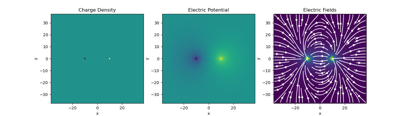
mesh.plot_image(rho, v_type="CC", ax=ax1)
ax1.set_title("Charge Density")

ax2 = fig.add_subplot(132)
mesh.plot_image(phi, v_type="CC", ax=ax2)
ax2.set_title("Electric Potential")

ax3 = fig.add_subplot(133)
mesh.plot_image(
    E, ax=ax3, v_type="F", view="vec", stream_opts={"color": "w", "density": 1.0}
)
ax3.set_title("Electric Fields")

Text(0.5, 1.0, 'Electric Fields')