discretize.base.BaseMesh.nodal_gradient#
- property BaseMesh.nodal_gradient#
Nodal gradient operator (nodes to edges).
This property constructs the 2nd order numerical gradient operator that maps from nodes to edges. The operator is a sparse matrix \(\mathbf{G_n}\) that can be applied as a matrix-vector product to a discrete scalar quantity \(\boldsymbol{\phi}\) that lives on the nodes, i.e.:
grad_phi = Gn @ phi
Once constructed, the operator is stored permanently as a property of the mesh.
- Returns:
- (
n_edges,n_nodes)scipy.sparse.csr_matrix The numerical gradient operator from nodes to edges
- (
Notes
In continuous space, the gradient operator is defined as:
\[\vec{u} = \nabla \phi = \frac{\partial \phi}{\partial x}\hat{x} + \frac{\partial \phi}{\partial y}\hat{y} + \frac{\partial \phi}{\partial z}\hat{z}\]Where \(\boldsymbol{\phi}\) is the discrete representation of the continuous variable \(\phi\) on the nodes and \(\mathbf{u}\) is the discrete representation of \(\vec{u}\) on the edges, nodal_gradient constructs a discrete linear operator \(\mathbf{G_n}\) such that:
\[\mathbf{u} = \mathbf{G_n} \, \boldsymbol{\phi}\]The Cartesian components of \(\vec{u}\) are defined on their corresponding edges (x, y or z) as follows; e.g. the x-component of the gradient is defined on x-edges. For edge \(i\) which defines a straight path of length \(h_i\) between adjacent nodes \(n_1\) and \(n_2\):
\[u_i = \frac{\phi_{n_2} - \phi_{n_1}}{h_i}\]Note that \(u_i \in \mathbf{u}\) may correspond to a value on an x, y or z edge. See the example below.
Examples
Below, we demonstrate 1) how to apply the nodal gradient operator to a discrete scalar quantity, and 2) the mapping of the nodal gradient operator and its sparsity. Our example is carried out on a 2D mesh but it can be done equivalently for a 3D mesh.
We start by importing the necessary packages and modules.
>>> from discretize import TensorMesh
>>> import numpy as np
>>> import matplotlib.pyplot as plt
>>> import matplotlib as mpl
For a discrete scalar quantity defined on the nodes, we take the gradient by constructing the gradient operator and multiplying as a matrix-vector product.
Create a uniform grid
>>> h = np.ones(20)
>>> mesh = TensorMesh([h, h], "CC")
Create a discrete scalar on nodes
>>> nodes = mesh.nodes
>>> phi = np.exp(-(nodes[:, 0] ** 2 + nodes[:, 1] ** 2) / 4 ** 2)
Construct the gradient operator and apply to vector
>>> Gn = mesh.nodal_gradient
>>> grad_phi = Gn @ phi
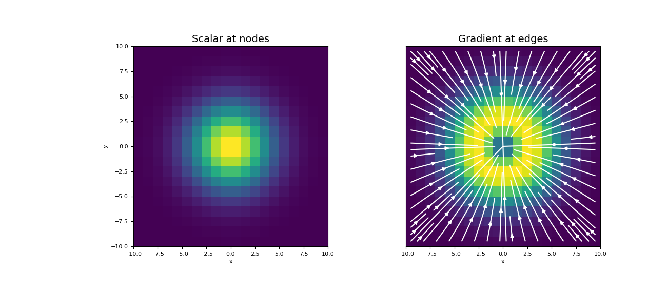
Plot the original function and the gradient
>>> fig = plt.figure(figsize=(13, 6))
>>> ax1 = fig.add_subplot(121)
>>> mesh.plot_image(phi, v_type="N", ax=ax1)
>>> ax1.set_title("Scalar at nodes", fontsize=14)
>>> ax2 = fig.add_subplot(122)
>>> mesh.plot_image(
...     grad_phi, ax=ax2, v_type="E", view="vec",
...     stream_opts={"color": "w", "density": 1.0}
... )
>>> ax2.set_yticks([])
>>> ax2.set_ylabel("")
>>> ax2.set_title("Gradient at edges", fontsize=14)
>>> plt.show()
(
Source code,png,pdf)
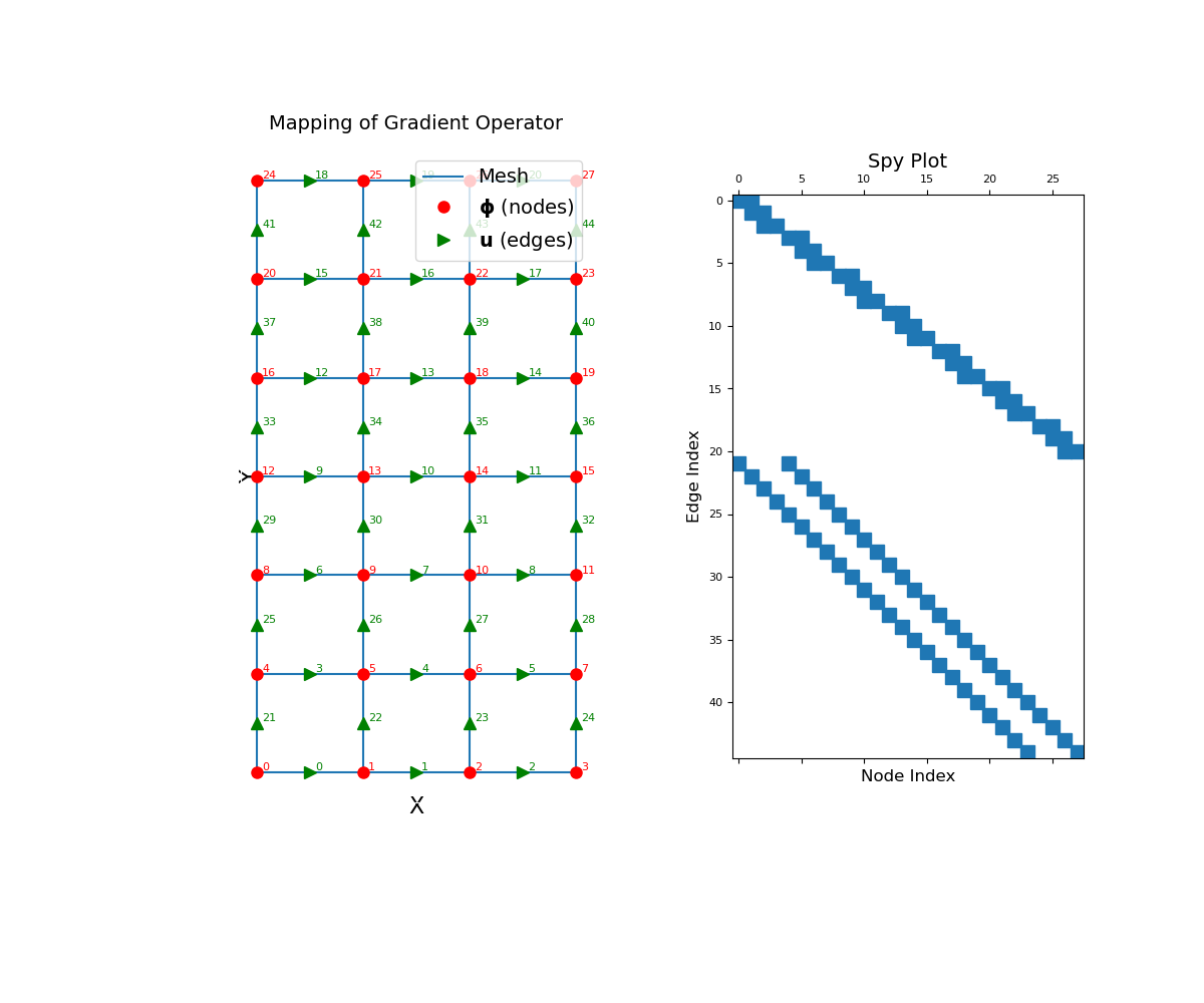
The nodal gradient operator is a sparse matrix that maps from nodes to edges. To demonstrate this, we construct a small 2D mesh. We then show the ordering of the elements in the original discrete quantity \(\boldsymbol{\phi}\) and its discrete gradient as well as a spy plot.
>>> mesh = TensorMesh([[(1, 3)], [(1, 6)]])
>>> fig = plt.figure(figsize=(12, 10))
>>> ax1 = fig.add_subplot(121)
>>> mesh.plot_grid(ax=ax1)
>>> ax1.set_title("Mapping of Gradient Operator", fontsize=14, pad=15)
>>> ax1.plot(mesh.nodes[:, 0], mesh.nodes[:, 1], "ro", markersize=8)
>>> for ii, loc in zip(range(mesh.nN), mesh.nodes):
>>>     ax1.text(loc[0] + 0.05, loc[1] + 0.02, "{0:d}".format(ii), color="r")
>>> ax1.plot(mesh.edges_x[:, 0], mesh.edges_x[:, 1], "g>", markersize=8)
>>> for ii, loc in zip(range(mesh.nEx), mesh.edges_x):
>>>     ax1.text(loc[0] + 0.05, loc[1] + 0.02, "{0:d}".format(ii), color="g")
>>> ax1.plot(mesh.edges_y[:, 0], mesh.edges_y[:, 1], "g^", markersize=8)
>>> for ii, loc in zip(range(mesh.nEy), mesh.edges_y):
>>>     ax1.text(loc[0] + 0.05, loc[1] + 0.02, "{0:d}".format((ii + mesh.nEx)), color="g")
>>> ax1.set_xticks([])
>>> ax1.set_yticks([])
>>> ax1.spines['bottom'].set_color('white')
>>> ax1.spines['top'].set_color('white')
>>> ax1.spines['left'].set_color('white')
>>> ax1.spines['right'].set_color('white')
>>> ax1.set_xlabel('X', fontsize=16, labelpad=-5)
>>> ax1.set_ylabel('Y', fontsize=16, labelpad=-15)
>>> ax1.legend(
>>>     ['Mesh', r'$\mathbf{\phi}$ (nodes)', r'$\mathbf{u}$ (edges)'],
>>>     loc='upper right', fontsize=14
>>> )
>>> ax2 = fig.add_subplot(122)
>>> ax2.spy(mesh.nodal_gradient)
>>> ax2.set_title("Spy Plot", fontsize=14, pad=5)
>>> ax2.set_ylabel("Edge Index", fontsize=12)
>>> ax2.set_xlabel("Node Index", fontsize=12)
>>> plt.show()
