discretize.base.BaseRectangularMesh.average_node_to_cell#

property BaseRectangularMesh.average_node_to_cell#

Averaging operator from nodes to cell centers (scalar quantities).

This property constructs a 2nd order averaging operator that maps scalar quantities from nodes to cell centers. This averaging operator is used when a discrete scalar quantity defined on mesh nodes must be projected to cell centers. Once constructed, the operator is stored permanently as a property of the mesh. See notes.

Returns:

(n_cells, n_nodes) scipy.sparse.csr_matrix

The scalar averaging operator from nodes to cell centers

Notes

Let ${\mathit{\varphi }}_{\mathit{n}}$ be a discrete scalar quantity that lives on mesh nodes. average_node_to_cell constructs a discrete linear operator ${\mathbf{A}}_{\mathbf{nc}}$ that projects ${\mathit{\varphi }}_{\mathit{f}}$ to cell centers, i.e.:

$${\mathit{\varphi }}_{\mathit{c}}={\mathbf{A}}_{\mathbf{nc}}{\mathit{\varphi }}_{\mathit{n}}$$

where ${\mathit{\varphi }}_{\mathit{c}}$ approximates the value of the scalar quantity at cell centers. For each cell, we are simply averaging the values defined on its nodes. The operation is implemented as a matrix vector product, i.e.:

phi_c = Anc @ phi_n

Examples

Here we compute the values of a scalar function on the nodes. We then create an averaging operator to approximate the function at cell centers. We choose to define a scalar function that is strongly discontinuous in some places to demonstrate how the averaging operator will smooth out discontinuities.

We start by importing the necessary packages and defining a mesh.

>>> from discretize import TensorMesh
>>> import numpy as np
>>> import matplotlib.pyplot as plt
>>> h = np.ones(40)
>>> mesh = TensorMesh([h, h], x0="CC")

Then we Create a scalar variable on nodes

>>> phi_n = np.zeros(mesh.nN)
>>> xy = mesh.nodes
>>> phi_n[(xy[:, 1] > 0)] = 25.0
>>> phi_n[(xy[:, 1] < -10.0) & (xy[:, 0] > -10.0) & (xy[:, 0] < 10.0)] = 50.0

Next, we construct the averaging operator and apply it to the discrete scalar quantity to approximate the value at cell centers.

>>> Anc = mesh.average_node_to_cell
>>> phi_c = Anc @ phi_n

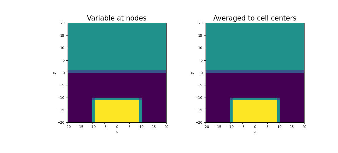
Plot the results,

>>> fig = plt.figure(figsize=(11, 5))
>>> ax1 = fig.add_subplot(121)
>>> mesh.plot_image(phi_n, ax=ax1, v_type="N")
>>> ax1.set_title("Variable at nodes", fontsize=16)
>>> ax2 = fig.add_subplot(122)
>>> mesh.plot_image(phi_c, ax=ax2, v_type="CC")
>>> ax2.set_title("Averaged to cell centers", fontsize=16)
>>> plt.show()

(Source code, png, pdf)

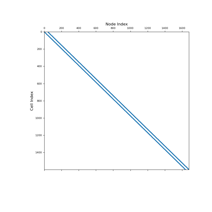
Below, we show a spy plot illustrating the sparsity and mapping of the operator

>>> fig = plt.figure(figsize=(9, 9))
>>> ax1 = fig.add_subplot(111)
>>> ax1.spy(Anc, ms=1)
>>> ax1.set_title("Node Index", fontsize=12, pad=5)
>>> ax1.set_ylabel("Cell Index", fontsize=12)
>>> plt.show()

(png, pdf)