Note
Go to the end to download the full example code.
Advanced Examples#
In this section, we demonstrate how to go from the inner product to the discrete approximation for some special cases. We also show how all necessary operators are constructed for each case.
Import Packages#
Here we import the packages required for this tutorial
from discretize.utils import sdiag
from discretize import TensorMesh
import numpy as np
import matplotlib.pyplot as plt

rng = np.random.default_rng(4321)
Constitive Relations and Differential Operators#
Where \(\psi\) and \(\phi\) are scalar quantities, \(\vec{u}\) and \(\vec{v}\) are vector quantities, and \(\sigma\) defines a constitutive relationship, we may need to derive discrete approximations for the following inner products:
\((\vec{u} , \sigma \nabla \phi)\)
\((\psi , \sigma \nabla \cdot \vec{v})\)
\((\vec{u} , \sigma \nabla \times \vec{v})\)
These cases effectively combine what was learned in the previous two tutorials. For each case, we must:
Define discretized quantities at the appropriate mesh locations
Define an inner product matrix that depends on a single constitutive parameter (\(\sigma\)) or a tensor (\(\Sigma\))
Construct differential operators that may require you to define boundary conditions
Where \(\mathbf{M_e}(\sigma)\) is the property dependent inner-product matrix for quantities on cell edges, \(\mathbf{M_f}(\sigma)\) is the property dependent inner-product matrix for quantities on cell faces, \(\mathbf{G_{ne}}\) is the nodes to edges gradient operator and \(\mathbf{G_{cf}}\) is the centers to faces gradient operator:
Where \(\mathbf{M_c}(\sigma)\) is the property dependent inner-product matrix for quantities at cell centers and \(\mathbf{D}\) is the faces to centers divergence operator:
Where \(\mathbf{C_{ef}}\) is the edges to faces curl operator and \(\mathbf{C_{fe}}\) is the faces to edges curl operator:
With the operators constructed below, you can compute all of the aforementioned inner products.
# Make basic mesh
h = np.ones(10)
mesh = TensorMesh([h, h, h])
sig = rng.random(mesh.nC)  # isotropic
Sig = rng.random((mesh.nC, 6))  # anisotropic

# Inner product matricies
Mc = sdiag(mesh.cell_volumes * sig)  # Inner product matrix (centers)
# Mn = mesh.getNodalInnerProduct(sig)  # Inner product matrix (nodes)  (*functionality pending*)
Me = mesh.get_edge_inner_product(sig)  # Inner product matrix (edges)
Mf = mesh.get_face_inner_product(sig)  # Inner product matrix for tensor (faces)

# Differential operators
Gne = mesh.nodal_gradient  # Nodes to edges gradient
mesh.set_cell_gradient_BC(
    ["neumann", "dirichlet", "neumann"]
)  # Set boundary conditions
Gcf = mesh.cell_gradient  # Cells to faces gradient
D = mesh.face_divergence  # Faces to centers divergence
Cef = mesh.edge_curl  # Edges to faces curl
Cfe = mesh.edge_curl.T  # Faces to edges curl

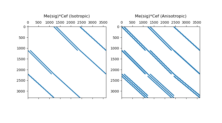
# EXAMPLE: (u, sig*Curl*v)
fig = plt.figure(figsize=(9, 5))

ax1 = fig.add_subplot(121)
ax1.spy(Mf * Cef, markersize=0.5)
ax1.set_title("Me(sig)*Cef (Isotropic)", pad=10)

Mf_tensor = mesh.get_face_inner_product(Sig)  # inner product matrix for tensor
ax2 = fig.add_subplot(122)
ax2.spy(Mf_tensor * Cef, markersize=0.5)
ax2.set_title("Me(sig)*Cef (Anisotropic)", pad=10)

Text(0.5, 1.082305057745918, 'Me(sig)*Cef (Anisotropic)')
Divergence of a Scalar and a Vector Field#
Where \(\psi\) and \(\phi\) are scalar quantities, and \(\vec{u}\) is a known vector field, we may need to derive a discrete approximation for the following inner product:
Scalar and vector quantities are generally discretized to lie on different locations on the mesh. As result, it is better to use the identity \(\nabla \cdot \phi \vec{u} = \phi \nabla \cdot \vec{u} + \vec{u} \cdot \nabla \phi\) and separate the inner product into two parts:
Term 1:
If the vector field \(\vec{u}\) is divergence free, there is no need to evaluate the first inner product term. This is the case for advection when the fluid is incompressible.
Where \(\mathbf{D_{fc}}\) is the faces to centers divergence operator, and \(\mathbf{M_c}\) is the basic inner product matrix for cell centered quantities, we can approximate this inner product as:
Term 2:
Let \(\mathbf{G_{cf}}\) be the cell centers to faces gradient operator, \(\mathbf{M_c}\) be the basic inner product matrix for cell centered quantities, and \(\mathbf{\tilde{A}_{fc}}\) and averages and sums the cartesian contributions of \(\vec{u} \cdot \nabla \phi\), we can approximate the inner product as:
With the operators constructed below, you can compute all of the inner products.
# Make basic mesh
h = np.ones(10)
mesh = TensorMesh([h, h, h])

# Inner product matricies
Mc = sdiag(mesh.cell_volumes * sig)  # Inner product matrix (centers)

# Differential operators
mesh.set_cell_gradient_BC(
    ["neumann", "dirichlet", "neumann"]
)  # Set boundary conditions
Gcf = mesh.cell_gradient  # Cells to faces gradient
Dfc = mesh.face_divergence  # Faces to centers divergence

# Averaging and summing matrix
Afc = mesh.dim * mesh.aveF2CC
Total running time of the script: (0 minutes 0.180 seconds)
