Note

Go to the end to download the full example code.

Constitutive Relations#

When solving PDEs using the finite volume approach, inner products may contain constitutive relations; examples include Ohm’s law and Hooke’s law. For this class of inner products, you will learn how to:

Construct the inner-product matrix in the case of isotropic and anisotropic constitutive relations

Construct the inverse of the inner-product matrix

Work with constitutive relations defined by the reciprocal of a parameter

Let $\vec{J}$ and $\vec{E}$ be two physically related quantities. If their relationship is isotropic (defined by a constant $σ$ ), then the constitutive relation is given by:

\vec{J} = σ \vec{E}

The inner product between a vector $\vec{v}$ and the right-hand side of this expression is given by:

(\vec{v}, σ \vec{E}) = \int_{Ω} \vec{v} \cdot σ \vec{E} d v

Just like in the previous tutorial, we would like to approximate the inner product numerically using an inner-product matrix such that:

(\vec{v}, σ \vec{E}) \approx v^{T} M_{σ} e

where the inner product matrix $M_{σ}$ now depends on:

the dimensions and discretization of the mesh

where $v$ and $e$ live

the spatial distribution of the property $σ$

In the case of anisotropy, the constitutive relations are defined by a tensor ( $Σ$ ). Here, the constitutive relation is of the form:

\vec{J} = Σ \vec{E}

where

\begin{array}{r} Σ = [\begin{array}{c} σ_{1} & σ_{4} & σ_{5} \\ σ_{4} & σ_{2} & σ_{6} \\ σ_{5} & σ_{6} & σ_{3} \end{array}] \end{array}

Is symmetric and defined by 6 independent parameters. The inner product between a vector $\vec{v}$ and the right-hand side of this expression is given by:

(\vec{v}, Σ \vec{E}) = \int_{Ω} \vec{v} \cdot Σ \vec{E} d v

Once again we would like to approximate the inner product numerically using an inner-product matrix $M_{Σ}$ such that:

(\vec{v}, Σ \vec{E}) \approx v^{T} M_{Σ} e

Import Packages#

Here we import the packages required for this tutorial

from discretize import TensorMesh
import numpy as np
import matplotlib.pyplot as plt

rng = np.random.default_rng(87236)

# sphinx_gallery_thumbnail_number = 1

Inner Product for a Single Cell#

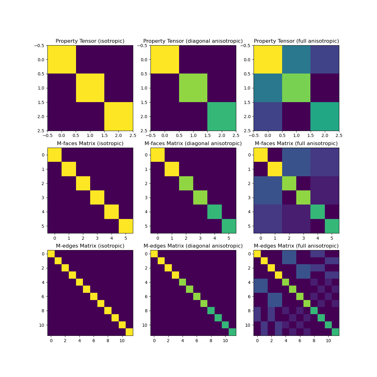
Here we compare the inner product matricies for a single cell when the constitutive relationship is:

isotropic: $σ_{1} = σ_{2} = σ_{3} = σ$ and $σ_{4} = σ_{5} = σ_{6} = 0$ ; e.g. $\vec{J} = σ \vec{E}$

diagonal anisotropic: independent parameters $σ_{1}, σ_{2}, σ_{3}$ and $σ_{4} = σ_{5} = σ_{6} = 0$

fully anisotropic: independent parameters $σ_{1}, σ_{2}, σ_{3}, σ_{4}, σ_{5}, σ_{6}$

When approximating the inner product according to the finite volume approach, the constitutive parameters are defined at cell centers; even if the fields/fluxes live at cell edges/faces. As we will see, inner-product matricies are generally diagonal; except for in the fully anisotropic case where the inner product matrix contains a significant number of non-diagonal entries.

# Create a single 3D cell
h = np.ones(1)
mesh = TensorMesh([h, h, h])

# Define 6 constitutive parameters for the cell
sig1, sig2, sig3, sig4, sig5, sig6 = 6, 5, 4, 3, 2, 1

# Isotropic case
sig = sig1 * np.ones((1, 1))
sig_tensor_1 = np.diag(sig1 * np.ones(3))
Me1 = mesh.get_edge_inner_product(sig)  # Edges inner product matrix
Mf1 = mesh.get_face_inner_product(sig)  # Faces inner product matrix

# Diagonal anisotropic
sig = np.c_[sig1, sig2, sig3]
sig_tensor_2 = np.diag(np.array([sig1, sig2, sig3]))
Me2 = mesh.get_edge_inner_product(sig)
Mf2 = mesh.get_face_inner_product(sig)

# Full anisotropic
sig = np.c_[sig1, sig2, sig3, sig4, sig5, sig6]
sig_tensor_3 = np.diag(np.array([sig1, sig2, sig3]))
sig_tensor_3[(0, 1), (1, 0)] = sig4
sig_tensor_3[(0, 2), (2, 0)] = sig5
sig_tensor_3[(1, 2), (2, 1)] = sig6
Me3 = mesh.get_edge_inner_product(sig)
Mf3 = mesh.get_face_inner_product(sig)

# Plotting matrix entries
fig = plt.figure(figsize=(12, 12))

ax1 = fig.add_subplot(331)
ax1.imshow(sig_tensor_1)
ax1.set_title("Property Tensor (isotropic)")

ax2 = fig.add_subplot(332)
ax2.imshow(sig_tensor_2)
ax2.set_title("Property Tensor (diagonal anisotropic)")

ax3 = fig.add_subplot(333)
ax3.imshow(sig_tensor_3)
ax3.set_title("Property Tensor (full anisotropic)")

ax4 = fig.add_subplot(334)
ax4.imshow(Mf1.todense())
ax4.set_title("M-faces Matrix (isotropic)")

ax5 = fig.add_subplot(335)
ax5.imshow(Mf2.todense())
ax5.set_title("M-faces Matrix (diagonal anisotropic)")

ax6 = fig.add_subplot(336)
ax6.imshow(Mf3.todense())
ax6.set_title("M-faces Matrix (full anisotropic)")

ax7 = fig.add_subplot(337)
ax7.imshow(Me1.todense())
ax7.set_title("M-edges Matrix (isotropic)")

ax8 = fig.add_subplot(338)
ax8.imshow(Me2.todense())
ax8.set_title("M-edges Matrix (diagonal anisotropic)")

ax9 = fig.add_subplot(339)
ax9.imshow(Me3.todense())
ax9.set_title("M-edges Matrix (full anisotropic)")

Property Tensor (isotropic), Property Tensor (diagonal anisotropic), Property Tensor (full anisotropic), M-faces Matrix (isotropic), M-faces Matrix (diagonal anisotropic), M-faces Matrix (full anisotropic), M-edges Matrix (isotropic), M-edges Matrix (diagonal anisotropic), M-edges Matrix (full anisotropic)

Text(0.5, 1.0, 'M-edges Matrix (full anisotropic)')

Spatially Variant Parameters#

In practice, the parameter $σ$ or tensor $Σ$ will vary spatially. In this case, we define the parameter $σ$ (or parameters $Σ$ ) for each cell. When creating the inner product matrix, we enter these parameters as a numpy array. This is demonstrated below. Properties of the resulting inner product matricies are discussed.

# Create a small 3D mesh
h = np.ones(5)
mesh = TensorMesh([h, h, h])

# Isotropic case: (nC, ) numpy array
sig = rng.random(mesh.nC)  # sig for each cell
Me1 = mesh.get_edge_inner_product(sig)  # Edges inner product matrix
Mf1 = mesh.get_face_inner_product(sig)  # Faces inner product matrix

# Linear case: (nC, dim) numpy array
sig = rng.random((mesh.nC, mesh.dim))
Me2 = mesh.get_edge_inner_product(sig)
Mf2 = mesh.get_face_inner_product(sig)

# Anisotropic case: (nC, 3) for 2D and (nC, 6) for 3D
sig = rng.random((mesh.nC, 6))
Me3 = mesh.get_edge_inner_product(sig)
Mf3 = mesh.get_face_inner_product(sig)

# Properties of inner product matricies
print("\n FACE INNER PRODUCT MATRIX")
print("- Number of faces              :", mesh.nF)
print("- Dimensions of operator       :", str(mesh.nF), "x", str(mesh.nF))
print("- Number non-zero (isotropic)  :", str(Mf1.nnz))
print("- Number non-zero (linear)     :", str(Mf2.nnz))
print("- Number non-zero (anisotropic):", str(Mf3.nnz), "\n")

print("\n EDGE INNER PRODUCT MATRIX")
print("- Number of faces              :", mesh.nE)
print("- Dimensions of operator       :", str(mesh.nE), "x", str(mesh.nE))
print("- Number non-zero (isotropic)  :", str(Me1.nnz))
print("- Number non-zero (linear)     :", str(Me2.nnz))
print("- Number non-zero (anisotropic):", str(Me3.nnz), "\n")

 FACE INNER PRODUCT MATRIX
- Number of faces              : 450
- Dimensions of operator       : 450 x 450
- Number non-zero (isotropic)  : 450
- Number non-zero (linear)     : 450
- Number non-zero (anisotropic): 3450


 EDGE INNER PRODUCT MATRIX
- Number of faces              : 540
- Dimensions of operator       : 540 x 540
- Number non-zero (isotropic)  : 540
- Number non-zero (linear)     : 540
- Number non-zero (anisotropic): 4140

Inverse#

The final discretized system using the finite volume method may contain the inverse of the inner-product matrix. Here we show how to call this using the invert_matrix keyword argument.

For the isotropic and diagonally anisotropic cases, the inner product matrix is diagonal. As a result, its inverse can be easily formed. For the full anisotropic case however, we cannot expicitly form the inverse because the inner product matrix contains a significant number of off-diagonal elements.

For the isotropic and diagonal anisotropic cases we can form $M^{- 1}$ then apply it to a vector using the $*$ operator. For the full anisotropic case, we must form the inner product matrix and do a numerical solve.

# Create a small 3D mesh
h = np.ones(5)
mesh = TensorMesh([h, h, h])

# Isotropic case: (nC, ) numpy array
sig = rng.random(mesh.nC)
Me1_inv = mesh.get_edge_inner_product(sig, invert_matrix=True)
Mf1_inv = mesh.get_face_inner_product(sig, invert_matrix=True)

# Diagonal anisotropic: (nC, dim) numpy array
sig = rng.random((mesh.nC, mesh.dim))
Me2_inv = mesh.get_edge_inner_product(sig, invert_matrix=True)
Mf2_inv = mesh.get_face_inner_product(sig, invert_matrix=True)

# Full anisotropic: (nC, 3) for 2D and (nC, 6) for 3D
sig = rng.random((mesh.nC, 6))
Me3 = mesh.get_edge_inner_product(sig)
Mf3 = mesh.get_face_inner_product(sig)

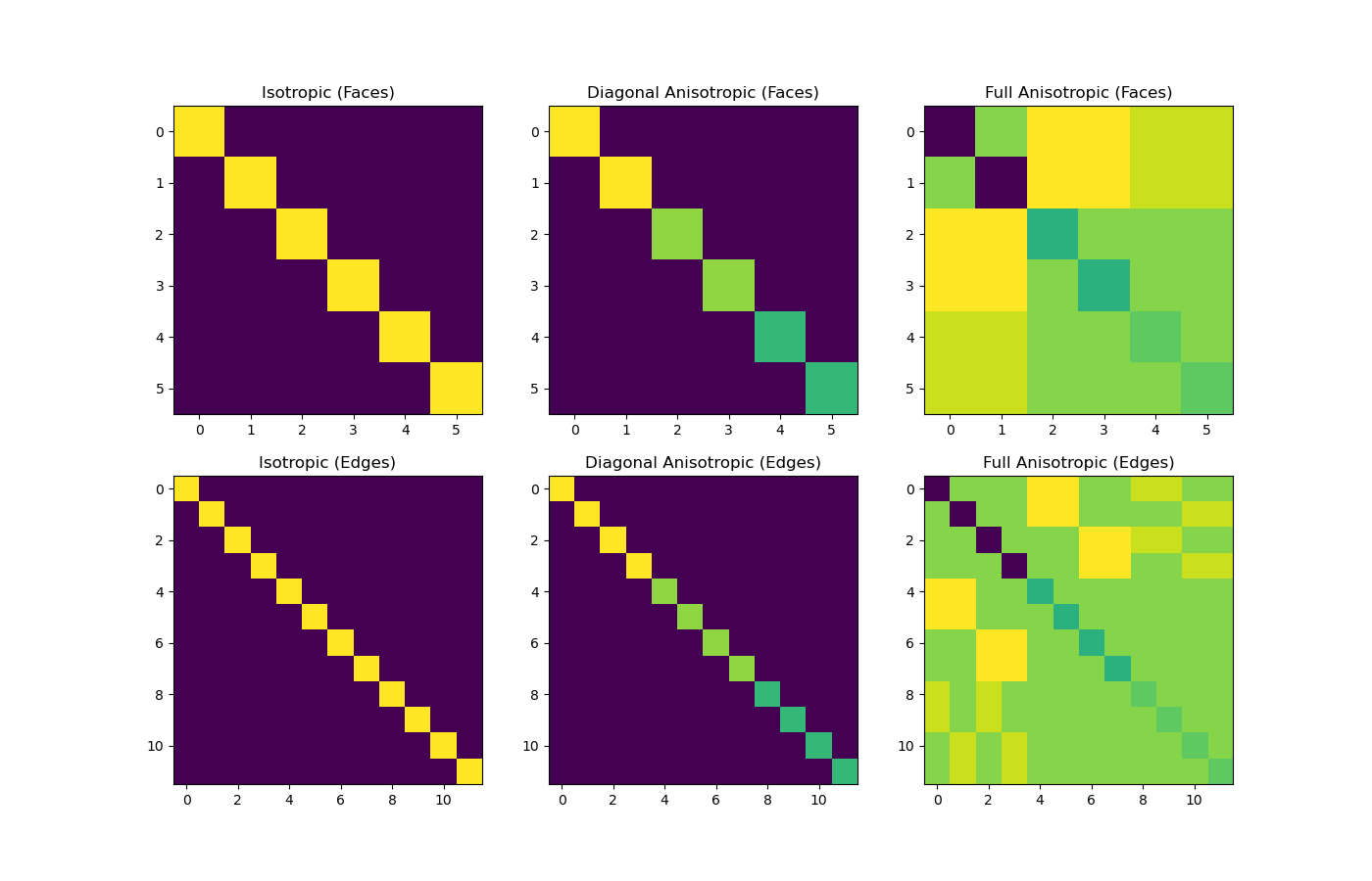
Reciprocal Properties#

At times, the constitutive relation may be defined by the reciprocal of a parameter ( $ρ$ ). Here we demonstrate how inner product matricies can be formed using the keyword argument invert_model. We will do this for a single cell and plot the matrix elements. We can easily extend this to a mesh comprised of many cells.

In this case, the constitutive relation is given by:

\vec{J} = \frac{1}{ρ} \vec{E}

The inner product between a vector $\vec{v}$ and the right-hand side of the expression is given by:

(\vec{v}, ρ^{- 1} \vec{E}) = \int_{Ω} \vec{v} \cdot ρ^{- 1} \vec{E} d v

where the inner product is approximated using an inner product matrix $M_{ρ^{- 1}}$ as follows:

(\vec{v}, ρ^{- 1} \vec{E}) \approx v^{T} M_{ρ^{- 1}} e

In the case that the constitutive relation is defined by a tensor $P$ , e.g.:

\vec{J} = P \vec{E}

where

\begin{array}{r} P = [\begin{array}{c} ρ_{1}^{- 1} & ρ_{4}^{- 1} & ρ_{5}^{- 1} \\ ρ_{4}^{- 1} & ρ_{2}^{- 1} & ρ_{6}^{- 1} \\ ρ_{5}^{- 1} & ρ_{6}^{- 1} & ρ_{3}^{- 1} \end{array}] \end{array}

The inner product between a vector $\vec{v}$ and the right-hand side of this expression is given by:

(\vec{v}, P \vec{E}) = \int_{Ω} \vec{v} \cdot P \vec{E} d v

Once again we would like to approximate the inner product numerically using an inner-product matrix $M_{P}$ such that:

(\vec{v}, P \vec{E}) \approx v^{T} M_{P} e

Here we demonstrate how to form the inner-product matricies $M_{ρ^{- 1}}$ and $M_{P}$ .

# Create a small 3D mesh
h = np.ones(1)
mesh = TensorMesh([h, h, h])

# Define 6 constitutive parameters for the cell
rho1, rho2, rho3, rho4, rho5, rho6 = (
    1.0 / 6.0,
    1.0 / 5.0,
    1.0 / 4.0,
    1.0 / 3.0,
    1.0 / 2.0,
    1,
)

# Isotropic case
rho = rho1 * np.ones((1, 1))
Me1 = mesh.get_edge_inner_product(rho, invert_model=True)  # Edges inner product matrix
Mf1 = mesh.get_face_inner_product(rho, invert_model=True)  # Faces inner product matrix

# Diagonal anisotropic case
rho = np.c_[rho1, rho2, rho3]
Me2 = mesh.get_edge_inner_product(rho, invert_model=True)
Mf2 = mesh.get_face_inner_product(rho, invert_model=True)

# Full anisotropic case
rho = np.c_[rho1, rho2, rho3, rho4, rho5, rho6]
Me3 = mesh.get_edge_inner_product(rho, invert_model=True)
Mf3 = mesh.get_face_inner_product(rho, invert_model=True)

# Plotting matrix entries
fig = plt.figure(figsize=(14, 9))

ax1 = fig.add_subplot(231)
ax1.imshow(Mf1.todense())
ax1.set_title("Isotropic (Faces)")

ax2 = fig.add_subplot(232)
ax2.imshow(Mf2.todense())
ax2.set_title("Diagonal Anisotropic (Faces)")

ax3 = fig.add_subplot(233)
ax3.imshow(Mf3.todense())
ax3.set_title("Full Anisotropic (Faces)")

ax4 = fig.add_subplot(234)
ax4.imshow(Me1.todense())
ax4.set_title("Isotropic (Edges)")

ax5 = fig.add_subplot(235)
ax5.imshow(Me2.todense())
ax5.set_title("Diagonal Anisotropic (Edges)")

ax6 = fig.add_subplot(236)
ax6.imshow(Me3.todense())
ax6.set_title("Full Anisotropic (Edges)")

Isotropic (Faces), Diagonal Anisotropic (Faces), Full Anisotropic (Faces), Isotropic (Edges), Diagonal Anisotropic (Edges), Full Anisotropic (Edges)

Text(0.5, 1.0, 'Full Anisotropic (Edges)')

Total running time of the script: (0 minutes 0.819 seconds)

Gallery generated by Sphinx-Gallery