Note
Go to the end to download the full example code.
Cylindrical meshes#
Cylindrical meshes (CylindricalMesh) are defined in terms of r
(radial position), z (vertical position) and phi (azimuthal position).
They are a child class of the tensor mesh class. Cylindrical meshes are useful
in solving differential equations that possess rotational symmetry. Here we
demonstrate:
How to create basic cylindrical meshes
How to include padding cells
How to plot cylindrical meshes
How to extract properties from meshes
How to create cylindrical meshes to solve PDEs with rotational symmetry
Import Packages#
Here we import the packages required for this tutorial.
from discretize import CylindricalMesh
import matplotlib.pyplot as plt
import numpy as np
Basic Example#
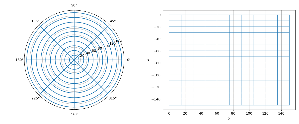
The easiest way to define a cylindrical mesh is to define the cell widths in r, phi and z as 1D numpy arrays. And to provide a Cartesian position for the bottom of the vertical axis of symmetry of the mesh. Note that
phi is in radians
The sum of values in the numpy array for phi cannot exceed \(2\pi\)
ncr = 10  # number of mesh cells in r
ncp = 8  # number of mesh cells in phi
ncz = 15  # number of mesh cells in z
dr = 15  # cell width r
dz = 10  # cell width z

hr = dr * np.ones(ncr)
hp = (2 * np.pi / ncp) * np.ones(ncp)
hz = dz * np.ones(ncz)

x0 = 0.0
y0 = 0.0
z0 = -150.0

mesh = CylindricalMesh([hr, hp, hz], x0=[x0, y0, z0])

mesh.plot_grid()

PolarAxes

[<PolarAxes: >, <Axes: xlabel='x', ylabel='z'>]
Padding Cells and Extracting Properties#
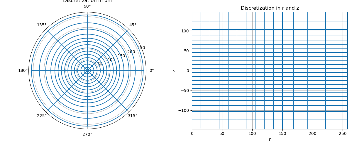
For practical purposes, the user may want to define a region where the cell widths are increasing/decreasing in size. For example, padding is often used to define a large domain while reducing the total number of mesh cells. Here we demonstrate how to create cylindrical meshes that have padding cells. We then show some properties that can be extracted from cylindrical meshes.
ncr = 10  # number of mesh cells in r
ncp = 8  # number of mesh cells in phi
ncz = 15  # number of mesh cells in z
dr = 15  # cell width r
dp = 2 * np.pi / ncp  # cell width phi
dz = 10  # cell width z
npad_r = 4  # number of padding cells in r
npad_z = 4  # number of padding cells in z
exp_r = 1.25  # expansion rate of padding cells in r
exp_z = 1.25  # expansion rate of padding cells in z

# Use a list of tuples to define cell widths in each direction. Each tuple
# contains the cell with, number of cells and the expansion factor (+ve/-ve).
hr = [(dr, ncr), (dr, npad_r, exp_r)]
hp = [(dp, ncp)]
hz = [(dz, npad_z, -exp_z), (dz, ncz), (dz, npad_z, exp_z)]

# We can use flags 'C', '0' and 'N' to define the xyz position of the mesh.
mesh = CylindricalMesh([hr, hp, hz], x0="00C")

# We can apply the plot_grid method and change the axis properties
ax = mesh.plot_grid()
ax[0].set_title("Discretization in phi")

ax[1].set_title("Discretization in r and z")
ax[1].set_xlabel("r")
ax[1].set_xbound(mesh.x0[0], mesh.x0[0] + np.sum(mesh.h[0]))
ax[1].set_ybound(mesh.x0[2], mesh.x0[2] + np.sum(mesh.h[2]))

# The bottom end of the vertical axis of rotational symmetry
x0 = mesh.x0

# The total number of cells
nC = mesh.nC

# An (nC, 3) array containing the cell-center locations
cc = mesh.gridCC

# The cell volumes
v = mesh.cell_volumes

PolarAxes
Cylindrical Mesh for Rotational Symmetry#
Cylindrical mesh are most useful when solving problems with perfect rotational symmetry. More precisely when:
field components in the phi direction are 0
fluxes in r and z are 0
In this case, the size of the forward problem can be significantly reduced. Here we demonstrate how to create a mesh for solving differential equations with perfect rotational symmetry. Since the fields and fluxes are independent of the phi position, there will be no need to discretize along the phi direction.
ncr = 10  # number of mesh cells in r
ncz = 15  # number of mesh cells in z
dr = 15  # cell width r
dz = 10  # cell width z
npad_r = 4  # number of padding cells in r
npad_z = 4  # number of padding cells in z
exp_r = 1.25  # expansion rate of padding cells in r
exp_z = 1.25  # expansion rate of padding cells in z

hr = [(dr, ncr), (dr, npad_r, exp_r)]
hz = [(dz, npad_z, -exp_z), (dz, ncz), (dz, npad_z, exp_z)]

# A value of 1 is used to define the discretization in phi for this case.
mesh = CylindricalMesh([hr, 1, hz], x0="00C")

# The bottom end of the vertical axis of rotational symmetry
x0 = mesh.x0

# The total number of cells
nC = mesh.nC

# An (nC, 3) array containing the cell-center locations
cc = mesh.gridCC

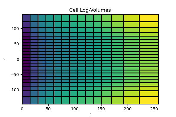
# Plot the cell volumes.
v = mesh.cell_volumes

fig = plt.figure(figsize=(6, 4))
ax = fig.add_subplot(111)
mesh.plot_image(np.log10(v), grid=True, ax=ax)
ax.set_xlabel("r")
ax.set_xbound(mesh.x0[0], mesh.x0[0] + np.sum(mesh.h[0]))
ax.set_ybound(mesh.x0[2], mesh.x0[2] + np.sum(mesh.h[2]))
ax.set_title("Cell Log-Volumes")

Text(0.5, 1.0, 'Cell Log-Volumes')
Notice that we do not plot the discretization in phi as it is irrelevant.
Total running time of the script: (0 minutes 0.500 seconds)
