Note
Go to the end to download the full example code.
Averaging Matricies#
Averaging matricies are used when a discrete variable living on some part of the mesh (e.g. nodes, centers, edges or faces) must be approximated at other locations. Averaging matricies are sparse and exist for 1D, 2D and 3D meshes. For each mesh class (Tensor mesh, Tree mesh, Curvilinear mesh), the set of averaging matricies are properties that are only constructed when called.
Here we discuss:
How to construct and apply averaging matricies
Averaging matricies in 1D, 2D and 3D
Averaging discontinuous functions
The transpose of an averaging matrix
Import Packages#
Here we import the packages required for this tutorial.
from discretize import TensorMesh
import matplotlib.pyplot as plt
import numpy as np

# sphinx_gallery_thumbnail_number = 3
1D Example#
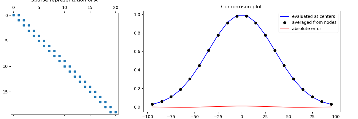
Here we compute a scalar function on cell nodes and average to cell centers. We then compute the scalar function at cell centers to validate the averaging operator.
# Create a uniform grid
h = 10 * np.ones(20)
mesh = TensorMesh([h], "C")

# Get node and cell center locations
x_nodes = mesh.nodes_x
x_centers = mesh.cell_centers_x


# Define a continuous function
def fun(x):
    return np.exp(-(x**2) / 50**2)


# Compute function on nodes and cell centers
v_nodes = fun(x_nodes)
v_centers = fun(x_centers)

# Create operator and average from nodes to cell centers
A = mesh.aveN2CC
v_approx = A * v_nodes

# Compare
fig = plt.figure(figsize=(12, 4))
ax1 = fig.add_axes([0.03, 0.01, 0.3, 0.91])
ax1.spy(A, markersize=5)
ax1.set_title("Sparse representation of A", pad=10)

ax2 = fig.add_axes([0.4, 0.06, 0.55, 0.85])
ax2.plot(
    x_centers,
    v_centers,
    "b-",
    x_centers,
    v_approx,
    "ko",
    x_centers,
    np.c_[v_centers - v_approx],
    "r-",
)
ax2.set_title("Comparison plot")
ax2.legend(("evaluated at centers", "averaged from nodes", "absolute error"))

fig.show()

1D, 2D and 3D Averaging#
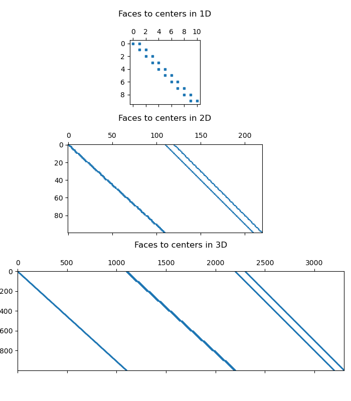
Here we discuss averaging operators in 1D, 2D and 3D. In 1D we can average between nodes and cell centers. In higher dimensions, we may need to average between nodes, cell centers, faces and edges. For this example we describe the averaging operator from faces to cell centers in 1D, 2D and 3D.
# Construct uniform meshes in 1D, 2D and 3D
h = 10 * np.ones(10)
mesh1D = TensorMesh([h], x0="C")
mesh2D = TensorMesh([h, h], x0="CC")
mesh3D = TensorMesh([h, h, h], x0="CCC")

# Create averaging operators
A1 = mesh1D.aveF2CC  # Averages faces (nodes in 1D) to centers
A2 = mesh2D.aveF2CC  # Averages from x and y faces to centers
A3 = mesh3D.aveF2CC  # Averages from x, y and z faces to centers

# Plot sparse representation
fig = plt.figure(figsize=(7, 8))
ax1 = fig.add_axes([0.37, 0.72, 0.2, 0.2])
ax1.spy(A1, markersize=2.5)
ax1.set_title("Faces to centers in 1D", pad=17)

ax2 = fig.add_axes([0.17, 0.42, 0.6, 0.22])
ax2.spy(A2, markersize=1)
ax2.set_title("Faces to centers in 2D", pad=17)

ax3 = fig.add_axes([0.05, 0, 0.93, 0.4])
ax3.spy(A3, markersize=0.5)
ax3.set_title("Faces to centers in 3D", pad=17)

fig.show()

# Print some properties
print("\n For 1D mesh:")
print("- Number of cells:", str(mesh1D.nC))
print("- Number of faces:", str(mesh1D.nF))
print("- Dimensions of operator:", str(mesh1D.nC), "x", str(mesh1D.nF))
print("- Number of non-zero elements:", str(A1.nnz), "\n")

print("For 2D mesh:")
print("- Number of cells:", str(mesh2D.nC))
print("- Number of faces:", str(mesh2D.nF))
print("- Dimensions of operator:", str(mesh2D.nC), "x", str(mesh2D.nF))
print("- Number of non-zero elements:", str(A2.nnz), "\n")

print("For 3D mesh:")
print("- Number of cells:", str(mesh3D.nC))
print("- Number of faces:", str(mesh3D.nF))
print("- Dimensions of operator:", str(mesh3D.nC), "x", str(mesh3D.nF))
print("- Number of non-zero elements:", str(A3.nnz))

 For 1D mesh:
- Number of cells: 10
- Number of faces: 11
- Dimensions of operator: 10 x 11
- Number of non-zero elements: 20

For 2D mesh:
- Number of cells: 100
- Number of faces: 220
- Dimensions of operator: 100 x 220
- Number of non-zero elements: 400

For 3D mesh:
- Number of cells: 1000
- Number of faces: 3300
- Dimensions of operator: 1000 x 3300
- Number of non-zero elements: 6000
Discontinuous Functions and the Transpose#
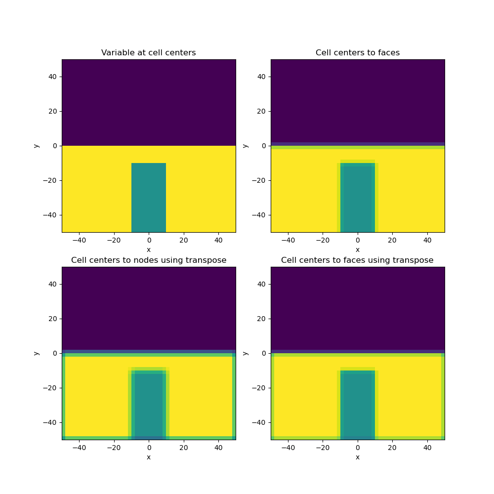
Here we show the effects of applying averaging operators to discontinuous functions. We will see that averaging smears the function at discontinuities.
The transpose of an averaging operator is also an averaging operator. For example, we can average from cell centers to faces by taking the transpose of operator that averages from faces to cell centers. Note that values on the boundaries are not accurate when applying the transpose as an averaging operator. This is also true for staggered grids.
# Create mesh and obtain averaging operators
h = 2 * np.ones(50)
mesh = TensorMesh([h, h], x0="CC")

A2 = mesh.aveCC2F  # cell centers to faces
A3 = mesh.aveN2CC  # nodes to cell centers
A4 = mesh.aveF2CC  # faces to cell centers

# Create a variable on cell centers
v = 100.0 * np.ones(mesh.nC)
xy = mesh.gridCC
v[(xy[:, 1] > 0)] = 0.0
v[(xy[:, 1] < -10.0) & (xy[:, 0] > -10.0) & (xy[:, 0] < 10.0)] = 50.0

fig = plt.figure(figsize=(10, 10))
ax1 = fig.add_subplot(221)
mesh.plot_image(v, ax=ax1)
ax1.set_title("Variable at cell centers")

# Apply cell centers to faces averaging
ax2 = fig.add_subplot(222)
mesh.plot_image(A2 * v, ax=ax2, v_type="F")
ax2.set_title("Cell centers to faces")

# Use the transpose to go from cell centers to nodes
ax3 = fig.add_subplot(223)
mesh.plot_image(A3.T * v, ax=ax3, v_type="N")
ax3.set_title("Cell centers to nodes using transpose")

# Use the transpose to go from cell centers to faces
ax4 = fig.add_subplot(224)
mesh.plot_image(A4.T * v, ax=ax4, v_type="F")
ax4.set_title("Cell centers to faces using transpose")

fig.show()

Total running time of the script: (0 minutes 0.422 seconds)
